---

• Description: GAVIS paper note: uncertainty quantification for 3DGS via a per-particle anisotropic visibility field; spherical harmonics representation, 200+ FPS real-time UQ, outperforms FisherRF/VIMC/NVF across all image-quality metrics
• My Notion Note ID: K2E-B-G2-7
• Created: 2026-07-01
• Updated: 2026-08-15
• License: Free to share: please credit Yu Zhang and link back to yuzhang.io

---

Table of Contents

• 1. Summary
• 2. Key Contributions
• 3. Background
• 4. Method
  • 4.1 Formulation
  • 4.2 Efficient Construction and Querying
  • 4.3 Active Mapping Pipeline
• 5. Experiments & Results
• 6. Ablation & Discussion
• 7. Strengths / Limitations / Future Work

---

1. Summary

Title: Uncertainty-driven 3D Gaussian Splatting Active Mapping via Anisotropic Visibility Field Authors: S. Xue*, J. Dill*, D. Ahuja*, F. Dellaert, P. Tsiotras, D. Xu (Georgia Institute of Technology) Paper: arXiv:2605.30342 (CVPR 2026) Github: xsj01/gavis · project page

GAVIS (Gaussian Splatting Anisotropic Visibility Field, Georgia Tech, 2026): an uncertainty quantification (UQ) and active-mapping framework for 3DGS (3D Gaussian Splatting, an explicit scene representation using Gaussian primitives).

Core problem: Active mapping (robot autonomously selects next viewpoint to maximize map quality) requires uncertainty estimates. Existing methods are either inaccurate or too slow. FisherRF and VIMC (Lyu et al. 2024, a Monte-Carlo manifold-sampling UQ method) give parametric UQ; NVF (Neural Visibility Field) learns an isotropic visibility field with a neural network and needs minutes of retraining per planning step.

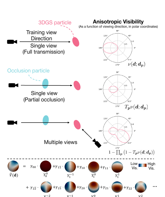
Key insight: Regions not covered by training views are inherently unreliable -> use visibility as a proxy for uncertainty. Unlike NVF's isotropic position function, GAVIS models anisotropic (direction-dependent) visibility: observing a Gaussian particle from one direction does not imply observing it from the opposite side (wall example). Visibility must be a function of render direction $\mathbf{d}$.

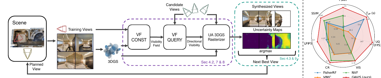
Main results: Outperforms FisherRF and VIMC across all four datasets (NeRF Synthetic / Space / Gibson / HM3D). Vs. NVF: dominant on image quality (PSNR/SSIM/LPIPS) and efficiency across all datasets; only Gibson mesh metrics (CR/VIS) slightly worse (HM3D: GAVIS edges NVF on CR 0.820 vs. 0.819, VIS 0.876 vs. 0.873). Visibility field built 500× faster than NVF (< 1 s vs. minutes); UQ at 200+ FPS. Works as a post-hoc plug-in: Fisher+GAVIS substantially improves FisherRF.

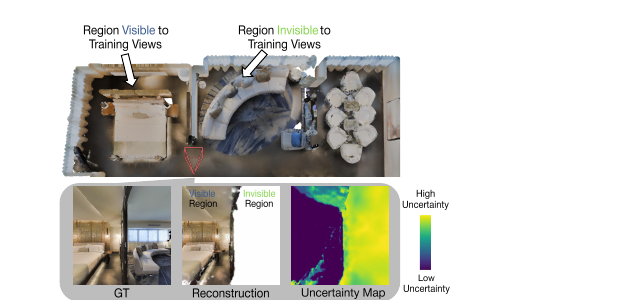
Reading note: the paper's main text is terse and defers most derivations and context to the appendix (Sec. 7). This note folds the key appendix results inline so it stands on its own: the entropy estimator (Eq. 30, 33), the SH construction and the AM-GM visibility bound (Sec. 7.1-7.3), and the visibility-compensated opacity (Eq. 27-28). To follow the method from the paper alone, plan on reading the appendix closely.

2. Key Contributions

• Anisotropic visibility field: per-particle direction-dependent visibility $V^{(i)}(\mathbf{d})$ with three factors (FOV indicator × transmittance × directional similarity, a von Mises-Fisher-style function); handles self-occlusion and multi-view coverage
• Efficient SH representation: $L=2$ spherical harmonics ($(L+1)^2 = 9$ params/particle) -> build complexity $O(|\mathcal{P}|)$, query $O(1)$ (independent of trajectory length); vs. naive SH representation at $O(|\mathcal{P}|^4 L^3)$ build cost
• Bayesian-network rasterizer: integrates visibility probability $v_i$ into a GMM pixel-color PDF; entropy used directly as active-mapping objective
• Virtual particles for density control: zero-opacity particles distinguish unexplored regions from free space -> high uncertainty assigned to unexplored areas
• General post-hoc module: plug into FisherRF or VIMC to substantially improve both

3. Background

Three preliminaries the method builds on (paper Sec. 3), kept in the paper's own equation order (NBV objective moved after the entropy machinery it depends on, for readability).

Radiance-field rendering (Eq. 1). A pixel color is the volume-rendering integral along its ray: accumulated color weighted by transmittance and density.

$$C(\mathbf{r}) = \int_{t_n}^{t_f} T(t)\,\sigma(t)\,\mathbf{c}(t)\,dt, \qquad T(t)=\exp\!\Bigl(-\!\int_{t_n}^{t}\sigma(s)\,ds\Bigr) \tag{1}$$

Symbols: $C(\mathbf{r})$ is the color of ray $\mathbf{r}$; $\sigma$ the density; $\mathbf{c}$ the emitted color; $T(t)$ the accumulated transmittance from the near bound $t_n$ to $t$. In practice the integral is discretized; 3DGS instantiates it with explicit Gaussian primitives.

Uncertainty-aware volume rendering (Eq. 3). A rendered pixel color is not one value but a distribution: standard 3DGS rendering returns its mean $\mathbb{E}[\mathbf{z}_0]$ (the image you see), while its spread (variance / entropy) is the uncertainty. GAVIS models that distribution as a visibility-gated GMM.

$$p(\mathbf{z}_0) = \sum_i w_i^*\,v_i\,\mathcal{N}(\boldsymbol{\mu}_{c_i}, \mathbf{Q}_{c_i}) + \mathcal{N}(\boldsymbol{\mu}_0, \mathbf{Q}_0)\sum_i w_i^*(1-v_i) \tag{3}$$

Symbols:

• $w_i^* = \alpha_i^*\prod_{j<i}(1-\alpha_j^*)$: the alpha-composite weight of particle $i$. This is the same per-particle contribution weight standard 3DGS already computes when rendering, here built from the visibility-compensated opacity $\alpha_i^*$ (paper Eq. 28).
• $v_i = V^{(i)}(\mathbf{d})$: visibility of particle $i$, in $[0,1]$ (defined in §4.1).
• $\mathcal{N}(\boldsymbol{\mu}_{c_i}, \mathbf{Q}_{c_i})$: particle $i$'s own color Gaussian. Base GAVIS sets a constant $\mathbf{Q}_{c_i}=\sigma_c^2\mathbf{I}$, since visibility (not the per-particle color variance) dominates the uncertainty.
• $\mathcal{N}(\boldsymbol{\mu}_0, \mathbf{Q}_0)$: a single shared "unobserved" prior with large variance $\mathbf{Q}_0$, i.e. maximum uncertainty.

Read it per particle (paper Eq. 27): each particle's weight $w_i^*$ is split by visibility. The $v_i$ share trusts the particle's own color $\mathcal{N}(\boldsymbol{\mu}_{c_i},\mathbf{Q}_{c_i})$; the $(1-v_i)$ share is handed to the default prior $\mathcal{N}(\boldsymbol{\mu}_0,\mathbf{Q}_0)$. That prior is identical for every unseen contribution, so it is factored out front and multiplies the total invisible weight $\sum_i w_i^*(1-v_i)$ (one shared component). Weight is conserved, $\sum_i w_i^* v_i + \sum_i w_i^*(1-v_i) = \sum_i w_i^*$: visibility only redistributes weight between "trust the color" and "fall back to the prior". Drop the second term and a never-observed pixel would collapse to zero weight or, after renormalizing, look falsely confident. The prior is where missing information goes, so low visibility widens the distribution.

Entropy readout. The pixel's uncertainty is the entropy of this distribution. Note that the paper's main text never writes the entropy out explicitly, but the generic definition is what you need to see where the estimator comes from. For any distribution,

$$\mathcal{H}(\mathbf{z}_0) = -\int p(\mathbf{z}_0)\,\log p(\mathbf{z}_0)\,d\mathbf{z}_0 \tag{S1}$$

Substitute the GMM $p(\mathbf{z}_0)$ of Eq. 3 into S1. A GMM's entropy has no closed form, so GAVIS bounds it with the Huber et al. upper bound (also adopted by NVF), used as an accurate estimator (paper Eq. 30):

$$\mathcal{H}(\mathbf{z}_0) \le \sum_{i=0}^{N} \bar{w}_i\Bigl(-\log \bar{w}_i + \tfrac{1}{2}\log\bigl((2\pi e)^{D}\,|\mathbf{Q}_i|\bigr)\Bigr) \tag{30}$$

with $\bar{w}_i := w_i^* v_i$ for $i\ge1$, the prior component $\bar{w}_0 := \sum_i w_i^*(1-v_i)$, $\mathbf{Q}_i := \mathbf{Q}_{c_i}$ ($i\ge1$) or $\mathbf{Q}_0$ ($i=0$), and $D=3$ (RGB channels). It has two parts:

• $-\log \bar{w}_i$: the mixing term, i.e. how spread the weights are across components.
• $\tfrac{1}{2}\log((2\pi e)^{D}|\mathbf{Q}_i|)$: each Gaussian's own entropy, which grows with its variance.

Low visibility puts more weight $\bar{w}_0$ on the huge-variance prior, so the entropy rises. This is accumulated per pixel inside the modified 3DGS rasterizer (hence real-time), then summed over the image with a spatial-correlation correction (paper Eq. 33) to give the view entropy $\mathcal{H}(\mathbf{Z}_\tau)$.

The chain. Visibility $v_i$ (§4) -> color distribution (Eq. 3) -> entropy (Eq. 30; generic definition S1) -> NBV selection (Eq. 2). Eq. 3 is the only place visibility enters the pixel model, and the entropy is a generic measure applied to whatever distribution Eq. 3 builds. That is the exact link between this GMM and the quantity $\mathcal{H}(\mathbf{Z}_\tau)$ that view selection maximizes.

Active mapping / NBV (Eq. 2). With $\mathcal{H}(\mathbf{Z}_\tau)$ now defined, next-best-view planning picks the candidate view of highest predicted observation entropy.

$$\tau^* = \arg\max_{\tau}\,\mathcal{H}(\mathbf{Z}_\tau) \tag{2}$$

Here $\tau$ is the candidate camera pose (action), $\mathbf{Z}_\tau$ the pixel-color observation from $\tau$ (a random variable), and $\mathcal{H}$ its entropy. This is the standard objective in radiance-field active mapping; GAVIS's contribution is the visibility that makes $\mathcal{H}$ trustworthy.

4. Method

4.1 Formulation

A quick primer on the kernel used below. The anisotropic factor is a von Mises-Fisher (vMF) function: the probability distribution over directions on the unit sphere. It belongs to a family that puts one idea (a peak at a mean, controlled by a spread parameter) on progressively higher-dimensional domains, each an analogue of the Gaussian:

Distribution	Domain	Density $\propto$	Parameters
Gaussian	real line, $x\in\mathbb{R}$	$\exp\!\bigl(-\tfrac{(x-\mu)^2}{2\sigma^2}\bigr)$	mean $\mu$, variance $\sigma^2$
von Mises	circle, angle $\theta$	$\exp\bigl(\kappa\cos(\theta-\mu)\bigr)$	mean angle $\mu$, concentration $\kappa$
von Mises-Fisher (vMF)	unit sphere, direction $\mathbf{x}$	$\exp(\kappa\,\boldsymbol{\mu}\cdot\mathbf{x})$	mean direction $\boldsymbol{\mu}$, concentration $\kappa$

In all three a larger spread parameter gives a tighter peak; the concentration $\kappa$ plays the role of $1/\sigma^2$ (large $\kappa$ = sharp, $\kappa=0$ = uniform, no preferred direction). GAVIS's directional kernel $\nu$ below is the vMF case with mean direction $\boldsymbol{\mu}=\mathbf{d}_p$ and $\mathbf{x}=\mathbf{d}$, so $\boldsymbol{\mu}\cdot\mathbf{x}=\mathbf{d}_p\cdot\mathbf{d}=\cos\theta$.

Single-view visibility (from camera pose $\mathbf{p}$ for particle $i$):

$$V^{(i)}_{\mathbf{p}}(\mathbf{d}) = \underbrace{\Phi_{i,\mathbf{p}}}_{\text{FOV}} \cdot \underbrace{T_{\mathbf{p}}(t_i^{\mathbf{p}})}_{\text{transmittance}} \cdot \underbrace{\nu(\mathbf{d};\,\mathbf{d}_p)}_{\text{dir. similarity}} \tag{4}$$

Three factors:

• $\Phi_{i,\mathbf{p}} \in \{0,1\}$: binary FOV indicator, i.e. whether particle $i$ falls inside camera $\mathbf{p}$'s field of view
• $T_{\mathbf{p}}(t_i^{\mathbf{p}})$: transmittance, the probability of reaching particle $i$ without occlusion along the ray from camera $\mathbf{p}$; read directly from the 3DGS rasterizer
• $\nu(\mathbf{d};\,\mathbf{d}_p) = \zeta\exp(\kappa\,\mathbf{d}\cdot\mathbf{d}_p)$: directional similarity, a vMF kernel with mean direction $\mathbf{d}_p$. Since $\mathbf{d}\cdot\mathbf{d}_p=\cos\theta$, it depends only on the angle $\theta$ between render and training directions, peaking when they align; $\zeta=\exp(-\kappa)$ is a constant that normalizes the peak so $\nu(\mathbf{d}_p;\mathbf{d}_p)=1$ (GAVIS normalizes the peak to 1 rather than integrating to 1, so $\nu$ is a vMF-shaped weight, not a strict density)

The first two terms $\Phi_{i,\mathbf{p}}\,T_{\mathbf{p}}(t_i^{\mathbf{p}})$ form an isotropic visibility (same as NVF); the third introduces directional anisotropy.

Full-dataset visibility (probability of being observed from at least one training view):

$$V^{(i)}(\mathbf{d}) = 1 - \prod_{\mathbf{p}\in\mathcal{P}}\!\bigl(1 - V^{(i)}_{\mathbf{p}}(\mathbf{d})\bigr) \tag{5}$$

$\mathcal{P}$: set of all observed camera poses.

4.2 Efficient Construction and Querying

Two naive approaches are unscalable:

• Direct product evaluation (Eq. 5 closed-form): must access all training view directions $\mathbf{d}_p$ at query time -> runtime and memory scale linearly with trajectory length $O(|\mathcal{P}|)$
• Naive SH representation of $V^{(i)}(\mathbf{d})$: SH-expand the total visibility directly. The catch: $V^{(i)}$ is a product over the $|\mathcal{P}|$ views (Eq. 5), and SH is linear only under addition: a product of two SH-expanded functions is not coefficient-wise. Multiplying two spherical harmonics couples their coefficients through triple products (Gaunt coefficients) and raises the truncation order, exactly like multiplying polynomials adds their degrees, or a product of Fourier series convolves their coefficients. Chaining $|\mathcal{P}|$ such factors makes the order (and coefficient count) grow with $|\mathcal{P}|$, and it is not incremental (a new frame forces a full recompute): build $O(|\mathcal{P}|^4 L^3)$, memory $O(|\mathcal{P}|^2 L^2)$, query $O(|\mathcal{P}|^2)$.

Both blow up as the trajectory grows. The fix follows from the same fact: SH stays cheap under a sum, so store an auxiliary sum (not the product) as a fixed-size SH field per particle, then recover the product from it.

Overview. Store each particle's visibility through an auxiliary field $\tilde{V}^{(i)}$ in truncated SH form, so construction is $O(|\mathcal{P}|)$ and query is $O(1)$:

$$\tilde{V}^{(i)}(\mathbf{d}) = \sum_{\ell=0}^{L}\sum_{m=-\ell}^{\ell} \gamma_{\ell m}^{\mathcal{P}}\,Y_{\ell}^m(\mathbf{d}) \tag{6}$$

Here $Y_{\ell}^m(\mathbf{d})$ are the spherical harmonics: a fixed orthonormal basis of functions on the direction sphere (the spherical analogue of a Fourier basis), indexed by degree $\ell$ (the band, $0\le\ell\le L$) and order $m$ ($-\ell\le m\le\ell$). $\gamma_{\ell m}^{\mathcal{P}}$ are the per-particle coefficients weighting each basis function, computed from the observed view set $\mathcal{P}$ (Eq. 11). Each particle stores $(L+1)^2 = 9$ coefficients (the paper finds $L=2$ sufficient to capture visibility; this is the same SH machinery original 3DGS uses for view-dependent color, though 3DGS color defaults to $L=3$). The rest of the section derives $\nu$'s SH form, then the coefficients $\gamma$ and the query bound.

SH representation of $\nu$. This is the same directional kernel $\nu = \zeta\exp(\kappa\,\mathbf{d}\cdot\mathbf{d}_p)$ from Eq. 4, only re-expressed in the fixed SH basis (an exact identity, not a new function), so its coefficients become additive across views and storable in fixed size. Because $\nu$ depends only on the angle between $\mathbf{d}$ and $\mathbf{d}_p$ (a zonal function on the sphere), the vMF has a closed-form SH expansion:

$$\nu(\mathbf{d};\mathbf{d}_p) = \zeta\sum_{\ell=0}^{\infty}\sum_{m=-\ell}^{\ell} a_{\ell m}\,Y_{\ell}^m(\mathbf{d}) \tag{7}$$ $$a_{\ell m} = 4\pi\,i_\ell(\kappa)\,Y_{\ell}^{m*}(\mathbf{d}_p) \tag{8}$$

$Y_{\ell}^m$: spherical harmonic basis; $i_\ell(\kappa)$: modified spherical Bessel function of the first kind; $Y_{\ell}^{m*}$: complex conjugate.

SH representation of $V^{(i)}$. $V^{(i)}$ is a product over views (Eq. 5), so it has no finite SH form directly. The trick is to bound it using only the auxiliary sum $\tilde{V}^{(i)}$, via the arithmetic-geometric-mean (AM-GM) inequality (geometric mean $\le$ arithmetic mean). With $a_{\mathbf{p}} := 1 - V^{(i)}_{\mathbf{p}} \in [0,1]$, AM-GM gives $\prod_{\mathbf{p}} a_{\mathbf{p}} \le \bigl(\tfrac{1}{|\mathcal{P}|}\sum_{\mathbf{p}} a_{\mathbf{p}}\bigr)^{|\mathcal{P}|}$; since $\sum_{\mathbf{p}} a_{\mathbf{p}} = |\mathcal{P}| - \tilde{V}^{(i)}$, substituting into Eq. 5 gives a lower bound that needs only $\tilde{V}^{(i)}$:

$$V^{(i)}(\mathbf{d}) \geq 1 - \Bigl(1 - \frac{\tilde{V}^{(i)}(\mathbf{d})}{|\mathcal{P}|}\Bigr)^{|\mathcal{P}|} \tag{9}$$

The bound is tight when all per-view $V^{(i)}_{\mathbf{p}}$ are equal (full derivation in the paper's appendix, Sec. 7.2-7.3). Being a lower bound, it underestimates visibility and so overestimates uncertainty, a safe bias for active mapping (explore a bit more rather than miss). Here the auxiliary field is the sum (not product) of per-view visibilities:

$$\tilde{V}^{(i)}(\mathbf{d}) := \sum_{\mathbf{p}} V^{(i)}_{\mathbf{p}}(\mathbf{d}) \tag{10}$$

and, substituting Eq. 7–8, its SH coefficients are computed analytically (no training):

$$\gamma_{\ell m}^{\mathcal{P}} = 4\pi\,\zeta\,i_\ell(\kappa)\!\sum_{\mathbf{p}\in\mathcal{P}}\Phi_{i,\mathbf{p}}\,T_{\mathbf{p}}(t_i^{\mathbf{p}})\,Y_{\ell}^{m*}(\mathbf{d}_p) \tag{11}$$

• Construction $O(|\mathcal{P}|)$: each new training frame accumulates its term $\Phi_{i,\mathbf{p}}\,T_{\mathbf{p}}(t_i^{\mathbf{p}})\,Y_{\ell}^{m*}(\mathbf{d}_p)$ into $\gamma_{\ell m}^{\mathcal{P}}$.
• Query $O(1)$: evaluate $\tilde{V}^{(i)}$ from the stored coefficients (Eq. 6), then the bound (Eq. 9), with no access to the training trajectory.

Density control: virtual particles. 3DGS adaptive density control prunes particles in empty regions. A "no particle" region can be either: ① free space (explored, pruned) or ② unexplored (insufficient initialization, zero gradient, never densified). Standard 3DGS cannot distinguish them, so particle-based UQ assigns low uncertainty to both, causing unexplored areas to be ignored.

Fix: uniformly sample virtual particles (zero opacity, not rendered) and compute their visibility. The contrast with a real particle is the point. A real particle's single-view visibility is anisotropic (Eq. 4),

$$V^{(i)}_{\mathbf{p}}(\mathbf{d}) = \Phi_{i,\mathbf{p}}\,T_{\mathbf{p}}(t_i^{\mathbf{p}})\,\nu(\mathbf{d};\mathbf{d}_p),$$

whereas a probe drops the directional term $\nu$ and keeps only $\Phi_{i,\mathbf{p}}\,T_{\mathbf{p}}(t_i^{\mathbf{p}})$ (isotropic, since a probe has no view-dependent appearance). Combined over all views this is Eq. 5 with $\nu\equiv1$ (the paper writes it inline, without an equation number):

$$V^{(i)}_\text{virtual}(\mathbf{d}) = 1 - \prod_{\mathbf{p}\in\mathcal{P}}\bigl(1-\Phi_{i,\mathbf{p}}\,T_{\mathbf{p}}(t_i^{\mathbf{p}})\bigr)$$

• Low-visibility virtual particle -> unexplored region -> keep, set $V^{(i)}(\mathbf{d}) = 0$ (maximum uncertainty)
• High-visibility virtual particle -> free space -> prune

Virtual particles ≈ 5–10% of total particle count; concatenated with trained 3DGS particles for UQ.

4.3 Active Mapping Pipeline

1. Train 3DGS on current observation frames
2. Build visibility field: analytically compute SH coefficients $\{\gamma_{\ell m}^{\mathcal{P}}\}$ for all particles (§4.2); add virtual particles
3. Candidate-view UQ: sample candidate poses $\tau$ from prior; compute the GMM entropy (Background, Eq. 3) via the uncertainty-aware rasterizer for each
4. Select NBV: $\tau^* = \arg\max \mathcal{H}(\mathbf{Z}_\tau)$ (Eq. 2); execute observation; repeat

Post-hoc plug-in mode: overlay GAVIS visibility $v_i$ onto existing UQ estimates (FisherRF, VIMC) to upweight low-visibility regions.

5. Experiments & Results

Settings: 3 domains, 4 datasets

• NeRF Synthetic (object reconstruction)
• Space dataset (Hubble HST + ISS)
• Gibson and HM3D (indoor home-robot environments, 8 scenes each)

Baselines:

• FisherRF: Fisher information UQ for 3DGS
• VIMC: Monte-Carlo manifold-sampling UQ (sampling-based variational inference; co-trains an uncertainty model)
• NVF: Neural Visibility Field, learns an isotropic visibility field for NeRF-based UQ

Metrics: PSNR/SSIM/LPIPS (image quality); CR (completion ratio, mesh coverage); VIS (visual coverage); $T_{UP}$ (uncertainty preparation time: visibility field build for GAVIS/NVF, Hessian estimation for FisherRF, training overhead for VIMC); UQ FPS (per candidate view)

Dataset	Method	PSNR ↑	SSIM ↑	LPIPS ↓	CR ↑	VIS ↑	UQ FPS ↑	$T_{UP}$ ↓
NeRF Syn.	FisherRF	22.34	0.870	0.119	0.626	0.376	146	0.42s
	VIMC	23.14	0.880	0.107	0.651	0.407	145	9.48s
	NVF	22.59	0.859	0.147	0.549	0.431	11.9	149.1s
	GAVIS	24.26	0.894	0.097	0.711	0.437	252	0.17s
Gibson	FisherRF	18.11	0.720	0.419	0.431	0.469	39.8	0.90s
	VIMC	15.70	0.668	0.465	0.337	0.366	57.0	90.5s
	NVF	23.29	0.798	0.402	0.880	0.915	4.2	219.9s
	GAVIS	24.42	0.812	0.323	0.831	0.890	207	0.42s

NVF beats GAVIS on CR/VIS only in Gibson (CR 0.880 vs. 0.831, VIS 0.915 vs. 0.890); on HM3D GAVIS edges NVF (CR 0.820 vs. 0.819, VIS 0.876 vs. 0.873). NVF trails on all image-quality metrics, UQ ≈30× slower on average (paper's headline figure; up to ~50× on Gibson/HM3D), visibility build ≈hundreds× slower. Space dataset: GAVIS PSNR 26.14 vs. NVF 23.76 (+2.4 dB), $T_{UP}$ 0.17s vs. 140.5s (826× speedup).

6. Ablation & Discussion

Ablation (Table 2, averaged over 4 datasets):

Configuration	PSNR ↑	SSIM ↑	LPIPS ↓	CR ↑	VIS ↑
Full GAVIS	24.70	0.839	0.224	0.748	0.697
Isotropic (no $\nu$ term)	23.97	0.827	0.231	0.741	0.671
No density control (no virtual particles)	24.18	0.830	0.234	0.712	0.668
Isotropic + no density control (≈ NVF ported to 3DGS)	23.38	0.819	0.240	0.691	0.625

Both components necessary: directional anisotropy contributes more to image quality (PSNR/SSIM/LPIPS); density control matters more for mesh coverage (CR/VIS). Isotropic + no density control (naive NVF->3DGS port) is worst.

Personal comment: the ablation deltas are small. Removing either component costs only about 0.5 to 0.7 dB PSNR, and dropping both about 1.3 dB. The table does establish that the two are necessary and complementary (anisotropy helps image quality, density control helps mesh coverage), but the effect sizes are modest. GAVIS's real edge over baselines is speed and uncertainty quality (AUSE), not large reconstruction gains from these two components. This is my own judgment; readers are welcome to weigh the numbers and form their own view.

GAVIS as post-hoc module (Table 3, averaged):

Method	PSNR ↑	SSIM ↑	LPIPS ↓	CR ↑	VIS ↑
FisherRF	20.73	0.779	0.285	0.513	0.469
FisherRF+GAVIS	24.70	0.842	0.220	0.748	0.699
VIMC	20.14	0.758	0.300	0.519	0.475
VIMC+GAVIS	24.21	0.833	0.227	0.719	0.672

FisherRF+GAVIS nearly matches standalone GAVIS (24.70 vs. 24.70) -> visibility modeling is the dominant factor in active mapping; parametric UQ adds little on top. VIMC+GAVIS slightly weaker, as VIMC's sampling noise interferes with the visibility signal.

Uncertainty quality (AUSE, 5 scenes). AUSE (Area Under the Sparsification Error curve) measures how well predicted uncertainty ranks the true errors: sort pixels by predicted uncertainty and progressively remove the most uncertain, then compare the resulting error-vs-fraction curve against the oracle curve (sorted by true error); the gap's area is AUSE (lower is better). It scores UQ ranking quality, not rendering accuracy:

Method	AUSE-D ↓	AUSE-V ↓
FisherRF	0.463	0.496
VIMC	0.504	0.447
NVF	0.381	0.231
GAVIS	0.224	0.176

AUSE-D (area under sparsification error curve by depth error) and AUSE-V (by visibility error, more aligned with active mapping goal) both best.

7. Strengths / Limitations / Future Work

Strengths

• Analytic visibility field: no neural network, built in < 1 s (NVF: minutes)
• 200+ FPS UQ -> real-time robot planning loop
• Outperforms all existing 3DGS UQ methods; composable as post-hoc module with any existing approach
• Virtual particles solve the UQ blind spot from 3DGS density pruning

Limitations

• Greedy single next-view: the action $\tau$ is restricted to the next camera pose; the expected information gain over an entire trajectory (joint entropy across a sequence of views) is not considered, which the paper calls an open challenge.
• Robot localization and dynamics uncertainty are not modeled; only the radiance field's own uncertainty is.
• Isotropic mesh metrics (CR/VIS) cannot fully credit anisotropic modeling: a mesh face counts as covered from any single direction, so these metrics do not reward revisiting a region from diverse viewpoints (paper's own point, §5.2 and appendix Sec. 12).

Personal comment: all experiments are on static scenes, so how the method behaves in dynamic environments is untested. This is my own observation, not a claim in the paper.

Future Work

• The paper notes the anisotropic visibility field is not limited to active mapping and could extend to other 3DGS tasks that require visibility estimation.