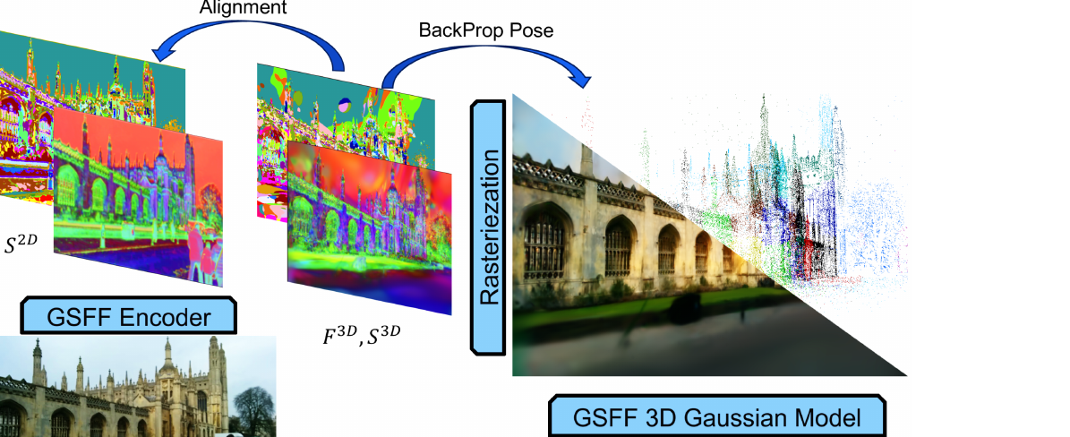
---

• Description: GSFF paper note. A per-scene representation fusing explicit 3DGS geometry with an implicit triplane feature field; a 2D encoder and the 3D field are aligned by contrastive losses, and structure-informed clustering turns features into segmentations for privacy-preserving visual localization by pose refinement.
• My Notion Note ID: K2E-B-G2-9
• Created: 2026-08-22
• Updated: 2026-08-22
• License: Free to share: please credit Yu Zhang and link back to yuzhang.io

---

Table of Contents

• 1. Paper Information
• 2. Summary
• 3. Key Contributions
• 4. Background
• 5. Method
  • 5.1 Scene Representation
  • 5.2 Prototypical Feature Regularization
  • 5.3 Feature-Based Localization (GSFFs-PR)
• 6. Privacy-Preserving GSFFs
• 7. Experimental Evaluation
  • 7.1 Visual Localization
  • 7.2 Ablations and Discussion
• 8. Conclusion

---

1. Paper Information

Title: Gaussian Splatting Feature Fields for Privacy-Preserving Visual Localization
Authors: Maxime Pietrantoni (Czech Technical University / CIIRC / NAVER LABS Europe), Gabriela Csurka (NAVER LABS Europe), Torsten Sattler (CIIRC, Czech Technical University)
Paper: arXiv:2507.23569 (CVPR 2025)
Github: no public code release found (as of 2026-08)

2. Summary

GSFF (Gaussian Splatting Feature Fields) is a per-scene representation for visual localization (VL), the task of estimating the 6-DoF camera pose of a query image in a known scene.

Core problem: feature-based VL leaks privacy. Recognizable scene images can be inverted from stored local descriptors, and cloud VL services expose both the user's query image and the scene map. The goal is a representation that localizes accurately yet reveals no privacy-sensitive appearance.

Core idea: fuse an explicit geometry model (3D Gaussian Splatting, specifically the Gaussian Opacity Fields / GoF variant, which gives accurate geometry) with an implicit feature field stored in a triplane grid (three axis-aligned 2D feature planes that parametrize a 3D field). Each Gaussian gets a scale-aware feature by projecting it onto the three planes with a covariance-based kernel. A jointly trained 2D image encoder and the 3D feature field are aligned in a shared space by contrastive losses. A structure-informed clustering step (spectral clustering on a Delaunay graph of Gaussian centers) produces prototypes, which both regularize the features and convert them to segmentation labels. Storing only geometry plus one integer label per Gaussian (dropping the feature field and the spherical-harmonic color) yields a privacy-preserving map.

Localization = pose refinement: from a retrieval-based initial pose, render the 3D feature (or segmentation) map from the GSFF and iteratively minimize the feature-metric (or segmentation cross-entropy) error over the pose by backpropagating through the rasterizer on SE(3). Two pipelines result: GSFFs-PR Feature (non-privacy) and GSFFs-PR Privacy (segmentation-based).

Main results: state of the art among 3DGS rendering-based and privacy-preserving methods on Cambridge Landmarks, 7Scenes, Indoor6, and 12Scenes; the privacy variant beats prior privacy baselines (SegLoc, GoMatch, DGC-GNN), often by large margins, and an image-inversion attack shows the privacy representation obfuscates scene appearance while the feature representation still leaks detail.

3. Key Contributions

• Gaussian Splatting Feature Fields: attach an implicit, triplane-parametrized feature field to an explicit 3DGS geometry, with a scale-aware per-Gaussian feature (large Gaussians aggregate features over a larger area, small ones over a smaller area).
• Self-supervised 3D-2D alignment: train, per scene, a 2D encoder and the 3D feature field jointly with contrastive losses so their features live in one embedding space; no manual labels.
• Structure-informed prototypes -> segmentations: spectral clustering on a Delaunay graph of Gaussian centers gives prototypes that regularize features and turn them into discrete segmentations.
• Privacy-preserving localization: pose refinement on segmentations (Gaussian geometry + integer labels only) reaches accuracy competitive with feature-based VL while resisting image-inversion attacks.

4. Background

3DGS rendering (Eq. 1). GSFF builds on Gaussian Opacity Fields (GoF), a 3DGS variant that integrates Mip-Splatting anti-aliasing and enforces accurate geometry through depth-distortion and normal-consistency regularization (important, since localization needs reliable 3D structure). A pixel color is the standard depth-ordered alpha composite over the Gaussians a ray traverses:

$$c(r,P)=\sum_{i=1}^{N} c_i\,\alpha_i\,C_i(r,P)\prod_{j=1}^{i-1}\bigl(1-\alpha_j\,C_j(r,P)\bigr) \tag{1}$$

Symbols: $r$ is the ray for a pixel at camera pose $P$; $c_i$ is the view-dependent color of Gaussian $G_i$ (from spherical harmonics); $\alpha_i$ its blending weight; $C_i(r,P)$ the Gaussian's contribution along the ray (the GoF ray-Gaussian intersection value); $N$ the depth-ordered Gaussians on the ray.

For readers new to GoF: it is a 3DGS variant built for accurate geometry, and the one change that buys that accuracy is how each Gaussian's contribution is measured. What makes this GoF rather than vanilla 3DGS is the term $C_i(r,P)$. Standard 3DGS projects each Gaussian to a 2D splat and weights it by that footprint evaluated at the pixel (an affine approximation of the projection, $\Sigma'=J\,W\,\Sigma\,W^{\top}J^{\top}$), which discards how the Gaussian's opacity varies with depth. GoF instead intersects the camera ray $x=o+t\,r$ with the 3D Gaussian: along the ray the Gaussian reduces to a 1D Gaussian in $t$ whose peak has a closed form at $t^{*}$, and $C_i(r,P)$ is that peak response. Because the evaluation stays in 3D, opacity is well-defined at any depth along the ray, giving a continuous opacity field whose level set is an accurate surface. That geometric fidelity (further sharpened by the depth-distortion and normal-consistency regularizers) is why GSFF builds on GoF: pose refinement needs reliable 3D structure and per-ray depth, which vanilla 3DGS's projected splats do not provide.

Features and segmentations are rendered by the same blending, replacing $c_i$ with the Gaussian's volumetric feature $g_i^{3D}$ (giving the feature map $F^{3D}$) or its one-hot label (giving the segmentation map $S^{3D}$).

5. Method

5.1 Scene Representation

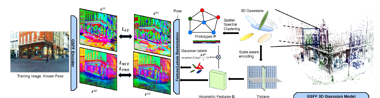
Storing an independent high-dimensional feature on every Gaussian is too costly, so GSFF parametrizes the implicit feature field by a triplane: three axis-aligned grids $H_{xy},H_{xz},H_{yz}\in\mathbb{R}^{R\times R\times D}$ (resolution $R$, feature dim $D$). These grids are the field's learnable parameters: a Gaussian does not carry its own feature, its scale-aware volumetric feature $g_i^{3D}$ is extracted from the triplane on demand. Training optimizes the three planes, and every Gaussian's feature is then assembled from them. For readers unfamiliar with triplanes: a dense 3D feature grid costs $O(R^3)$ memory, whereas a triplane keeps three 2D planes ($O(R^2)$ each) and reads a 3D point's feature by projecting it onto the three planes, sampling each, and combining, trading a little expressivity for a large memory saving. To extract that volumetric feature for a Gaussian $G_i$ (center $m_i$, covariance $\Sigma_i$), take one plane, say $xy$: (1) orthographically project the center to a 2D point $m_i^{xy}$ and the covariance to a 2D covariance $\Sigma_i^{xy}$ (dropping the off-plane axis); (2) place a $5\times5$ grid of offsets $u$ around $m_i^{xy}$; (3) query the feature plane $H_{xy}$ at each grid point and weight the queried features by a covariance-based RBF (radial basis function, a standard distance-decaying kernel) shaped by $\Sigma_i^{xy}$, i.e. a 2D Gaussian:

$$G_i^{xy}(u)=\tfrac{1}{Z}\exp\!\Bigl(-\tfrac{1}{2}\,u\,(\Sigma_i^{xy})^{-1}\,u^{\top}\Bigr)$$

Symbols: $u$ ranges over the $5\times5$ grid offsets around the projected center; $\Sigma_i^{xy}$ is the Gaussian's covariance projected to the $xy$ plane; $Z$ normalizes the kernel. The kernel-weighted sum over the 25 grid points gives the per-plane feature $g_i^{xy}$; repeating on the $xz$ and $yz$ planes and combining the three yields the volumetric feature $g_i^{3D}$. The feature is called scale-aware because the kernel is shaped by the Gaussian's own projected covariance $\Sigma_i^{xy}$: a Gaussian with large spatial span aggregates plane features over a large area of the grid and a small Gaussian over a smaller area. Sampling the plane only at the projected center instead would hand a large and a small Gaussian at the same location the identical feature, losing this scale information (the covariance kernel vs a point-wise projection is ablated in §7.2). Because projected footprints overlap, neighboring Gaussians share information, and the field is queryable at any 3D position, so it survives the split/merge of 3DGS densification.

Personal comment: the paper is inconsistent about the combine step, its main text (§3.1) says the three per-plane features are averaged while its appendix (A.3) says summed, and it does not confirm which was actually used. Sum and mean differ only by a global factor of three, which the learnable field and the loss temperature could plausibly absorb, so I would not expect it to change the result by much. This is my own reading, not a claim in the paper.

Personal comment: combining by sum/average at all (rather than concatenation) is the more interesting choice. It compresses the three $D$-dim plane features into a single $D$-dim vector (compact, but many-to-one, so distinct plane-feature triples can in principle collide), whereas concatenating them into a $3D$-dim vector would be collision-free at three times the storage. GSFF takes the compact option, which is where its "little expressivity" trade-off actually sits. This is my own reading, not a claim in the paper.

Self-supervised feature alignment.

Rendering the per-Gaussian volumetric features $g_i^{3D}$ (extracted from the triplane above) via Eq. 1, i.e. alpha-blending them along each ray in place of color, gives a 3D feature map $F^{3D}$ at the training pose. So $F^{3D}$ traces back to the triplane, carried by the Gaussians and rendered to the image; $F^{2D}$ comes from the separate 2D encoder. A per-scene 2D encoder, jointly trained with the field, produces $F^{2D}$ from the same image. Per the appendix, it has two levels: a coarse encoder (a pretrained DINOv2 backbone, followed by 1x1 projection convolutions that reduce the dimension, then a ConvNeXt block) and a fine encoder (shallow convolutions followed by a ConvNeXt block). The two are pulled together at each pixel with a symmetric InfoNCE-style contrastive loss (contrastive: pull the matched pair together, push all non-matching pairs apart):

$$L_{NCE}=-\frac{1}{2HW}\sum_{u\in I}\log\frac{\exp\!\bigl(F_u^{3D}\cdot F_u^{2D}/\tau\bigr)^2}{A} \tag{2}$$

Symbols: $u$ indexes pixels of the $H\times W$ map $I$; $F_u^{2D},F_u^{3D}$ are the aligned 2D/3D features; $\tau$ is a temperature. The similarity of a feature pair is their dot product $F^{3D}\cdot F^{2D}$, scaled by $\tau$. A single-direction term (fix $F_u^{3D}$ as the anchor) is a softmax over all pixels that pushes the matched pixel $u$ to dominate, pulling its own $F_u^{2D}$ closer and every other pixel's feature away; the symmetric loss adds this to its mirror (anchor $F_u^{2D}$, negatives over the 3D features). That is why the numerator is squared (the matched similarity appears in both directions) and $A$ is the product of the two directions' denominators (a 3D-to-2D sum and a 2D-to-3D sum, each over all pixels). The $2HW$ normalizes over the two directions and the $HW$ pixels. Matching pixels attract, non-matching repel, so the encoder and the field end up in one embedding space.

Multi-view consistency. To make features view-consistent and generalize to unseen viewpoints, a nearby pose is sampled, pixel correspondences are established by forward-backward reprojection through rendered depths (kept when the reprojection error is under a threshold), and for a random subset of the pixel-aligned pairs one side is replaced with the corresponding feature from the other view inside the contrastive terms.

5.2 Prototypical Feature Regularization

Spatial prototypes. A Delaunay triangulation of the Gaussian centers gives a sparse graph capturing local geometry. For readers unfamiliar: Delaunay triangulation connects a point set into a mesh of triangles (tetrahedra in 3D) such that no point falls inside any triangle's circumscribed circle; in effect it wires each Gaussian center to its natural spatial neighbors, yielding a sparse "who is adjacent to whom" graph without picking a distance threshold. A Laplacian eigen-decomposition followed by spectral clustering then groups the Gaussians into $K$ clusters (tractable, unlike a dense pairwise-distance matrix). For readers unfamiliar with spectral clustering: it clusters nodes in the space spanned by the graph Laplacian's leading eigenvectors, so grouping follows graph connectivity (which Gaussians are spatially linked) rather than raw coordinate distance, which is why it beats k-means on the centers (ablation, §7.2). Each prototype $p_k$ is the mean volumetric feature of its cluster, updated during training by an exponential moving average. A prototype is thus the center of one cluster in feature space, so the $K$ prototypes act as $K$ label-free classes and a Gaussian's segmentation label is just its nearest prototype (§6).

Personal comment: From my understanding, a prototype is best read as a self-discovered class whose identity starts geometric and turns semantic: it is seeded by purely spatial clustering (spectral clustering on the Gaussian centers), then drifts under the feature losses and gets re-assigned by the optimal transport below, so the final classes are feature-coherent rather than merely spatial. The paper states the initialization and the updates but does not frame it this way. This is my own reading, not a claim in the paper.

Prototypical loss. For each pixel-aligned pair, both the 2D and the 3D feature are pulled toward their shared assigned prototype:

$$L_{PRO}=-\frac{1}{N}\sum_{n=1}^{N}\log\frac{\exp\!\bigl((F_n^{3D}\cdot p_n + F_n^{2D}\cdot p_n)/\tau\bigr)}{B} \tag{3}$$

Symbols: $N$ pixel-aligned pairs; $F_n^{2D},F_n^{3D}$ the pair's features; $p_n$ the prototype assigned to the pair; $\tau$ temperature; $B$ a normalizer over all $K$ prototypes (again a product over the two directions). The pair-to-prototype assignment is solved as an optimal transport problem with the Sinkhorn-Knopp algorithm, with an entropy term that balances cluster sizes and prevents collapse. For readers new to optimal transport: OT is the lowest-cost matching between two distributions under fixed marginals, and Sinkhorn-Knopp solves an entropy-regularized version cheaply by alternately normalizing the rows and columns of the assignment matrix; the marginal constraint is what spreads pixels across all prototypes instead of letting them collapse onto a single cluster. This tightens intra-cluster compactness, separates clusters, and injects the 3D spatial prior into the 2D features.

5.3 Feature-Based Localization (GSFFs-PR)

Localization is pose refinement. For readers new to visual localization: the common paradigm is retrieve-then-refine, where image retrieval first finds the database image most similar to the query by a global descriptor (one vector per image, here DenseVLAD) and borrows its pose as a coarse initialization, then a refinement step optimizes that pose against the scene model. GSFF keeps retrieval deliberately weak (DenseVLAD) so the accuracy comes from its refinement, not a strong initializer, which keeps the comparison to competitors fair. The pose is then optimized to align the query encoder features with the features rendered from the Gaussians at the current pose:

$$P^{*}=\min_{P\in SE(3)}\bigl\|F^{2D}-F^{3D}(P,G)\bigr\|_2^{2} \tag{4}$$

Symbols: $P$ the camera pose, optimized on the Lie algebra $\mathfrak{se}(3)$ by explicitly backpropagating through the rasterizer; $G$ the Gaussians; $F^{3D}(P,G)$ the feature map rendered at pose $P$. This is render-and-compare pose refinement: the Gaussian rasterizer is differentiable in the pose, so the gradient of the per-pixel feature error flows back to the 6-DoF pose and updates it by gradient descent on the SE(3) manifold, with no explicit 2D-3D feature matching (contrast classic structure-based VL, which matches keypoints and solves PnP). The render-then-update loop runs coarse-then-fine: the coarse level uses smooth, low-detail features whose pose-error landscape has a wide basin, so even a weak initial pose slides to the right answer, and the fine level uses sharp features that give high precision once the pose is already close (the coarse-vs-fine feature/segmentation maps are visualized in Fig. 3, §7.1). High-distortion and sky regions are masked out.

6. Privacy-Preserving GSFFs

From features to segmentations. To turn the feature field into discrete classes, each Gaussian's feature is soft-assigned to the prototypes: a softmax of its similarities to the $K$ prototypes gives a $K$-way class distribution (pseudo-logits), and the same is done for the encoder features:

$$l^{3D}_{ik}=\frac{\exp(g_i^{\top}p_k)}{\sum_{k'}\exp(g_i^{\top}p_{k'})},\qquad l^{2D}_{ik}=\frac{\exp(f_i^{\top}p_k)}{\sum_{k'}\exp(f_i^{\top}p_{k'})}$$

A shallow segmentation head on the encoder predicts $S^{2D}$ directly, trained so encoder and rendered segmentations agree:

$$L_{CE}=-\sum_{u\in I}\mathbf{1}_u\cdot\bigl(\log S_u^{2D}+\log S_u^{3D}\bigr) \tag{5}$$

Symbols: $\mathbf{1}_u$ is the one-hot label of pixel $u$, taken from the same optimal-transport associations used by $L_{PRO}$ (so features and segmentation stay consistent); $S_u^{3D}$ is the rendered pseudo-logit vector (the per-Gaussian soft-assignments alpha-blended along the ray), $S_u^{2D}$ the segmentation-head output. The cross-entropy pulls both the encoder segmentation $S^{2D}$ (which a query image can produce on its own) and the rendered map segmentation $S^{3D}$ toward the same label, so at localization the two can be compared under one class convention (Eq. 6).

Privacy model and localization. At deployment each Gaussian is hard-assigned a single label $k^{*}=\arg\max_k l_{ik}$, and the triplane feature field, prototypes, spherical-harmonic color, and all photometric information are removed. The stored map is only the Gaussian geometry (no color) plus one integer per Gaussian, so it is far smaller and reveals only coarse geometry (deemed non-privacy-violating). Why this preserves privacy: a high-dimensional feature encodes appearance densely enough that a learned decoder can invert it back to a recognizable image (the inversion attack in §7.1), whereas an integer label carries only cluster membership, almost no appearance, so there is nothing to invert. Localization renders the label map $S^{3D}$ and refines the pose on the segmentation cross-entropy:

$$P^{*}=\min_{P\in SE(3)} \mathrm{CE}\bigl(S^{2D},\,S^{3D}_P\bigr) \tag{6}$$

No features or color are needed at query time, so neither the query nor the map exposes recognizable appearance.

7. Experimental Evaluation

Datasets: 7Scenes (two pseudo-ground-truth protocols, SfM and Depth-SLAM), Cambridge Landmarks, Indoor6, and 12Scenes. Metrics: median position error (cm), median rotation error (deg), and recall at 5cm/5deg indoors.

7.1 Visual Localization

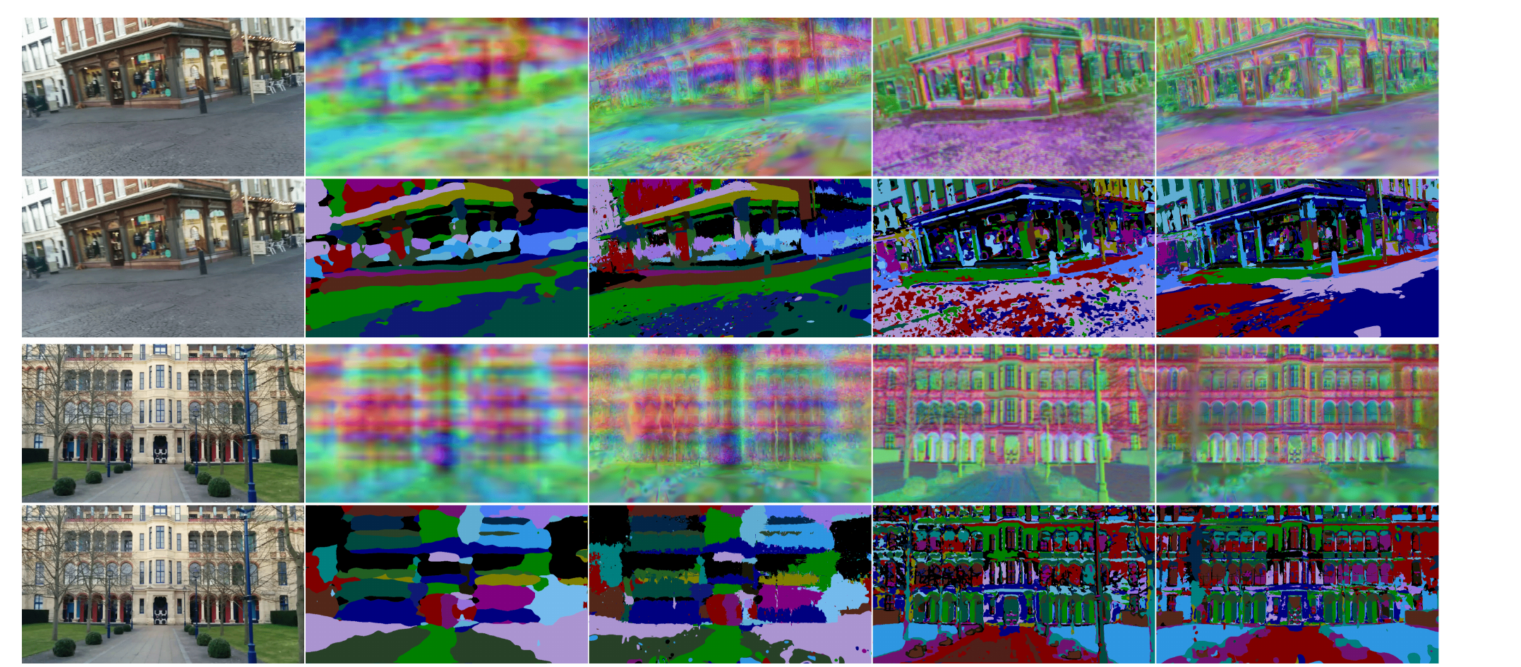
Cambridge Landmarks (outdoor, Table 2): GSFFs-PR Feature is the most accurate 3DGS rendering-based method (over GSplatLoc, GS-CPR, NeFeS, MCLoc) and competitive with structure-based methods, though the NeRF-based NeRFMatch stays ahead on King's College (13cm/0.2deg). Its tuned variant reaches King's College 17cm/0.26deg, Shop Facade 4cm/0.25deg, St Mary's 8cm/0.26deg (the untuned variant: 18/0.27, 4/0.26, 10/0.34). GSFFs-PR Privacy (e.g. King's 24cm/0.39deg, Shop 5cm/0.27deg) beats the privacy baseline SegLoc (a prior privacy method that localizes on a sparse SfM point cloud carrying per-point segmentation labels, contrasted with GSFF's dense rendered segmentation) by large margins on Old Hospital, Shop, and St Mary's.

Method	King's	Old Hosp.	Shop	St Mary's
SegLoc (privacy baseline)	24 / 0.26	36 / 0.52	11 / 0.34	17 / 0.46
GSFFs-PR Privacy	24 / 0.39	26 / 0.49	5 / 0.27	13 / 0.48
NeRFMatch	13 / 0.2	21 / 0.4	8.7 / 0.4	11.3 / 0.4
GSplatLoc	27 / 0.46	20 / 0.71	5 / 0.36	16 / 0.61
GSFFs-PR Feature	18 / 0.27	21 / 0.4	4 / 0.26	10 / 0.34
GSFFs-PR Feature (tuned)	17 / 0.26	18 / 0.36	4 / 0.25	8 / 0.26

Cells are median position error (cm) / median rotation error (deg); DenseVLAD initialization.

7Scenes (indoor): GSFFs-PR Feature is best on 4 of 7 scenes and second on 2 more despite a weaker initializer than DFNet/ACE (e.g. Chess 0.4cm/0.19deg, Fire 0.6cm/0.26deg, Redkitchen 0.6cm/0.23deg). It fails on Stairs (25.1cm) because the textureless, flat layout breaks the underlying Opacity Gaussian Field geometry. On the Depth-SLAM protocol the privacy variant beats SegLoc, GoMatch, and DGC-GNN on every scene.

Indoor6 (hard: multi-room, large illumination change): GSFFs-PR trained with 84 classes outperforms SegLoc in average recall; with 34 classes it is on par. More classes give more discriminative segmentations, which matters most for large, complex scenes.

Privacy / inversion attack: an image-inversion model is trained to reconstruct images from rendered maps. Reconstructions from GSFFs-PR Feature reveal substantial scene detail, whereas reconstructions from GSFFs-PR Privacy obfuscate privacy-sensitive appearance (qualitative, no privacy metric reported).

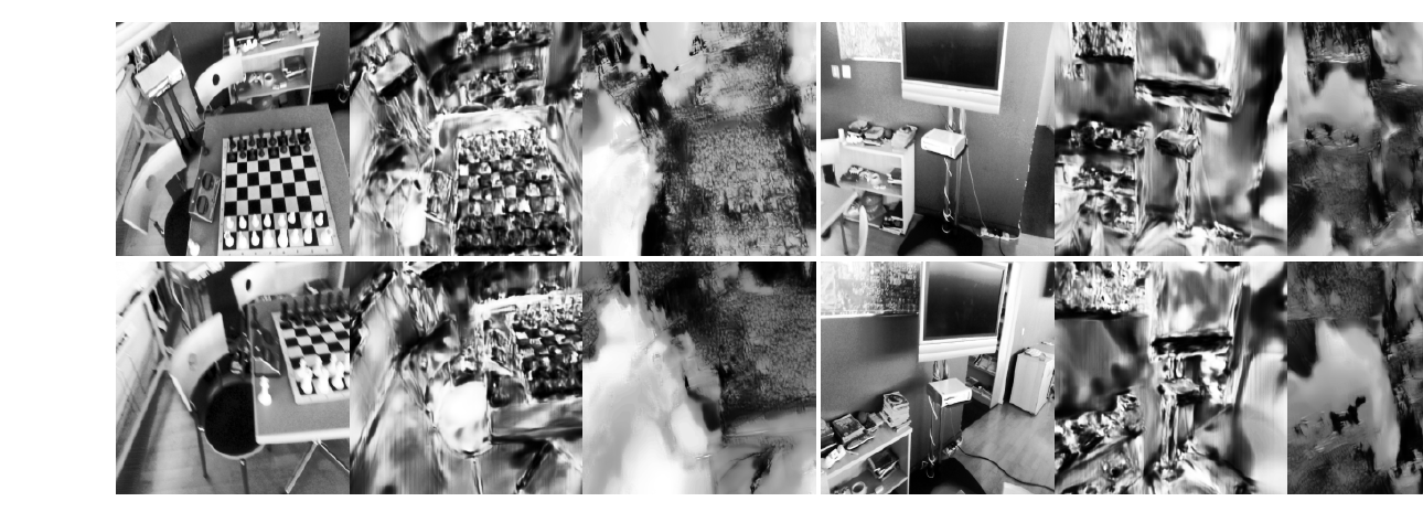
Cost: GSFF adds per-scene training time over plain GoF (about 10.8h vs 0.7h on Cambridge) but preserves novel-view-synthesis quality (PSNR/SSIM/LPIPS on par with GoF). A forward pass is about 0.024 to 0.046s; the backward pass used in pose optimization grows with the class count (34 vs 84 classes: about 0.065s vs 0.46s on King's), so 34 classes is a good speed/accuracy compromise. GSFFs-Privacy cannot render RGB by design.

7.2 Ablations and Discussion

On King's College and Old Hospital (Feature and Privacy), Table 5 (median position cm / rotation deg; KC = King's College, OH = Old Hospital, F = Feature, P = Privacy):

Variant	KC (F)	OH (F)	KC (P)	OH (P)
Coarse only	37.5 / 0.80	670 / 1.10	92.2 / 1.55	82.5 / 1.50
Fine only	22.6 / 0.32	55.1 / 0.77	28.0 / 0.45	151 / 0.96
k-means (vs spectral)	25.2 / 0.33	27.6 / 0.50	37.2 / 0.64	52.3 / 0.84
No segmentation head ($L_{CE}$)	23.5 / 0.30	23.4 / 0.45	31.0 / 0.45	30.8 / 0.57
No multi-view reg.	20.0 / 0.28	22.5 / 0.49	29.6 / 0.51	29.1 / 0.49
No scale-aware (point-wise)	23.5 / 0.31	21.9 / 0.42	27.0 / 0.42	26.0 / 0.47
Full GSFFs-PR	17.9 / 0.27	21.4 / 0.41	24.3 / 0.39	25.6 / 0.49

• Hierarchy: coarse-only is far worse (King's Feature 37.5cm), fine-only is worse than the full model (22.6cm); the full coarse-then-fine model reaches 17.9cm. The coarse level widens the convergence basin and the fine level sharpens accuracy.
• Clustering: replacing spectral clustering with k-means degrades accuracy (25.2 vs 17.9cm), so the structure-informed clustering matters.
• Scale-aware encoding: replacing the covariance kernel with a point-wise projection of Gaussian centers hurts (23.5cm).
• Multi-view regularization: removing the cross-view feature swapping hurts (20.0cm).
• Segmentation optimization: dropping $L_{CE}$ (soft assignments only) is noticeably worse (23.5cm); the explicit segmentation head both improves privacy localization and helps the feature alignment.
• Sparsity: refining on only the reprojected Gaussian centers (a SegLoc-style sparse signal) does not converge; a dense rendered signal is necessary when backpropagating through the renderer.
• Class count: too few prototypes are not discriminative, too many over-cluster and hurt convergence; larger scenes need more classes.

8. Conclusion

GSFF fuses explicit 3DGS geometry (GoF) with an implicit triplane feature field, aligns a per-scene 2D encoder and the 3D field self-supervised, and structures the space with geometry-seeded prototypes so features convert to segmentations. Localizing on segmentations (Gaussian geometry plus one integer label per Gaussian) reaches accuracy competitive with feature-based VL while resisting image-inversion attacks, and the added field preserves the base 3DGS novel-view-synthesis quality.

Limitations

• Textureless, flat scenes break the underlying geometry and the refinement (Stairs, 25.1cm).
• The number of segmentation classes must be tuned per scene: too few are not discriminative, too many hurt convergence.
• Refinement needs a dense rendered signal; a sparse signal does not converge through the renderer.
• The backward pass cost scales with class count, and GSFF adds substantial per-scene training time over plain GoF. The paper mentions combining low- and high-resolution refinement with early stopping to speed up localization but states no broader future-work agenda.

Personal comment: the privacy is argued only qualitatively (one inversion-attack figure, no metric), so it is shown by example rather than measured. Localization also still needs the per-scene 2D encoder to segment a query, an extra artifact that must be distributed, and whether its weights leak scene appearance is never analyzed. And the strong accuracy comes at a per-scene training cost (about 10.8h) and per-scene class tuning. This is my own reading, not a claim in the paper.