Description: Feature 3DGS paper note. Attach an optimizable semantic feature to every 3D Gaussian and render it with a parallel N-dimensional rasterizer, distilling 2D foundation-model features (SAM, CLIP-LSeg) into an explicit 3D feature field; a speed-up module renders a low-dim feature that a 1x1 conv lifts to the teacher dimension. Enables novel-view segmentation, SAM promptable segmentation from any view, and language-guided 3D editing.
My Notion Note ID: K2E-B-G2-8
Created: 2026-08-22
Updated: 2026-08-22
License: Free to share: please credit Yu Zhang and link back to yuzhang.io

1. Paper Information

Title: Feature 3DGS: Supercharging 3D Gaussian Splatting to Enable Distilled Feature Fields
Authors: Shijie Zhou, Haoran Chang*, Sicheng Jiang*, Zhiwen Fan, Zehao Zhu, Dejia Xu, Pradyumna Chari, Suya You, Zhangyang Wang, Achuta Kadambi (* equal contribution)
Affiliations: UCLA; UT Austin; DEVCOM Army Research Laboratory
Paper: arXiv:2312.03203 (CVPR 2024)
Github: feature-3dgs.github.io (project page); ShijieZhou-UCLA/feature-3dgs

2. Summary

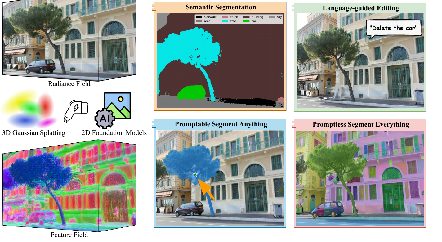
Feature 3DGS lifts 2D foundation-model features into an explicit 3D feature field built on 3D Gaussian Splatting (3DGS).

Core problem: 2D foundation models (SAM, CLIP-LSeg, DINO) produce rich per-pixel semantic features, and prior work distills them into 3D through NeRF-based feature fields (Distilled Feature Fields / N3F / LERF / NeRF-DFF). NeRF distillation is slow to render, and the implicit MLP produces continuity artifacts that hurt feature quality; sharing one radiance/feature MLP also forces a tiny feature-loss weight to avoid interference.

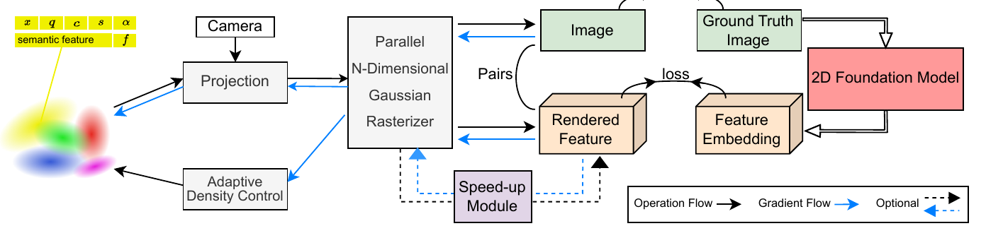
Core idea: attach an extra optimizable semantic feature $f\in\mathbb{R}^N$ to every 3D Gaussian (alongside position, covariance, opacity, color) and render it with a parallel N-dimensional Gaussian rasterizer that alpha-composites features exactly like colors, at the same spatial resolution as the RGB image. The rendered student feature map is distilled from a teacher 2D foundation-model embedding by an L1 loss, jointly with the photometric loss. Because the representation is explicit (not a shared MLP), the two losses can be weighted equally with no interference. To keep high-dimensional rendering fast, a speed-up module renders a low-dim feature ( $N\ll M$ , the teacher dimension) and a lightweight 1x1 convolution lifts the channels back to $M$ .

Downstream: novel-view semantic segmentation, SAM point/box promptable segmentation from any view (decode the rendered feature directly, skipping the SAM image encoder), and language-guided 3D editing (extract, delete, recolor by querying the feature field). It is the first method to enable point- and box-prompting for radiance-field manipulation.

Main results: on Replica, semantic-segmentation mIoU 0.787 vs NeRF-DFF 0.636 (about +23%) with higher accuracy; the speed-up module more than doubles feature-render FPS at negligible quality cost; up to about 2.7x faster feature distillation/rendering than the NeRF-based method; and adding the feature even improves RGB quality over vanilla 3DGS.

Feature 3DGS teaser (paper Fig. 1): one representation spans a radiance field and a distilled feature field, supporting novel-view semantic segmentation, language-guided editing ("delete the car"), and SAM promptable / promptless segmentation.

3. Key Contributions

Per-Gaussian feature + parallel N-dim rasterizer: add an optimizable semantic feature to each Gaussian and jointly render RGB and feature at matching spatial resolution (differing only in channel count), rather than a separate low-resolution feature pass.
Speed-up module: render a low-dim feature and lift it to the teacher dimension with a learnable 1x1 convolution, avoiding the cost of rendering full high-dim features while adding channel-wise mixing.
Explicit, interference-free distillation: because features live on Gaussians (not a shared MLP), the feature and photometric losses are equally weighted, avoiding the NeRF-DFF sensitivity to a tiny feature weight.
Promptable and editable 3D: SAM point/box segmentation from any view and language-guided 3D editing operating directly on Gaussians (so occluded parts can still be handled).

4. Background

Feature 3DGS keeps the 3DGS geometry. Each scene is a set of anisotropic 3D Gaussians initialized from an SfM (structure-from-motion) sparse point cloud. A Gaussian is projected to screen space by transforming its 3D covariance $\Sigma$ into a 2D covariance $\Sigma'$ :

\Sigma' = J\,W\,\Sigma\,W^{\top}J^{\top} \tag{1}

Symbols: $W$ is the world-to-camera transform; $J$ the Jacobian of the affine approximation of the projective transform; $\Sigma$ the 3D covariance, $\Sigma'$ the 2D screen-space covariance. To keep $\Sigma$ a valid (positive semi-definite) covariance during optimization, it is decomposed into rotation and scaling:

\Sigma = R\,S\,S^{\top}R^{\top} \tag{2}

Symbols: $R$ is a rotation matrix (stored as a unit quaternion $q\in\mathbb{R}^4$ ); $S$ a diagonal scaling matrix (stored as a scale $s\in\mathbb{R}^3$ ). Color uses spherical harmonics (introduced band by band during training). Feature 3DGS adds one attribute to this set: the semantic feature $f\in\mathbb{R}^N$ .

5. Method

5.1 High-Dimensional Semantic Feature Rendering

The rasterizer alpha-composites, front to back, both color and feature over the depth-sorted Gaussians hitting a pixel:

C=\sum_{i\in\mathcal{N}} c_i\,\alpha_i\,T_i,\qquad F_s=\sum_{i\in\mathcal{N}} f_i\,\alpha_i\,T_i \tag{3}

where $\mathcal{N}$ is the set of depth-sorted Gaussians overlapping the pixel and $T_i=\prod_{j=1}^{i-1}(1-\alpha_j)$ is the accumulated transmittance. Symbols: $C$ is the rendered pixel color and $F_s$ the rendered student feature ( $s$ = student, supervised by the teacher); $c_i,f_i,\alpha_i$ the color, semantic feature, and opacity of Gaussian $i$ . The two share the same tile-based rasterization and differ only in channel count, so the feature map is produced at the full image resolution in one joint pass, not a separate low-resolution stage.

5.2 Optimization and Speed-Up

A teacher 2D foundation model encodes each training image into a target feature map $F_t(I)\in\mathbb{R}^{H\times W\times M}$ ( $M=512$ for CLIP-LSeg, $256$ for SAM). Training minimizes the photometric loss plus an L1 feature-distillation loss:

L=L_{rgb}+\gamma\,L_f \tag{4}

with the photometric term $L_{rgb}=(1-\lambda)\,L_1(I,\hat I)+\lambda\,L_{\text{D-SSIM}}(I,\hat I)$ and the distillation term $L_f=\bigl\|F_t(I)-F_s(\hat I)\bigr\|_1$ . Symbols: $I$ the ground-truth image, $\hat I$ the rendered image; $F_t(I)$ the teacher embedding, $F_s(\hat I)$ the rendered student feature (bilinearly resized to $H\times W$ ); $\gamma$ the feature-loss weight (set to 1.0, equal weighting); $\lambda$ the SSIM mix (0.2), where D-SSIM is the structural-dissimilarity term $(1-\text{SSIM})/2$ . The equal weighting is possible because the feature lives on explicit Gaussians. NeRF-DFF instead routes radiance and feature through one shared MLP, so a large $\gamma$ drags the shared weights and corrupts the radiance; $\gamma$ must be kept tiny, which caps feature quality.

Speed-up module. Rendering cost scales with the channel count, since alpha-compositing an $N$ -dim vector over the depth-sorted Gaussians of each pixel is $O(N)$ work per Gaussian, so a full $M$ -dim feature is slow. The field instead renders a low-dim feature $f\in\mathbb{R}^N$ with $N\ll M$ , and a lightweight convolutional decoder with a 1x1 kernel lifts the channels $N\to M$ afterwards; the distillation L1 in Eq. 4 is computed on this lifted $M$ -dim map, not on the raw $N$ -dim render. It is cheap (the 1x1 conv acts on the small rendered $H\times W$ map, outside the per-Gaussian compositing loop), learnable (adds channel-wise mixing), and optional (dropping it and rendering $N=M$ directly does not hurt downstream quality). The lift works because it is trained jointly, as an autoencoder: the 1x1 conv is a per-pixel linear map $\mathbb{R}^N\to\mathbb{R}^M$ optimized so that $\text{conv}(F_s^N)$ reconstructs the teacher, which is possible because the teacher's $M$ -dim features are redundant (low intrinsic dimension); $N$ is a learned compressed code, not a lossy downsample. In practice $N=128$ (half of SAM's 256, a quarter of LSeg's 512), where mIoU already saturates (§6.4).

5.3 Promptable Explicit Scene Representation

Because every Gaussian carries a feature, prompts act directly in 3D. A prompt $\tau$ (a text query or a point) is embedded to $q(\tau)$ in feature space, and its activation on Gaussian $x$ is the cosine similarity:

s=\frac{f(x)\cdot q(\tau)}{\|f(x)\|\,\|q(\tau)\|} \tag{5}

Scores over a candidate label set $T$ are normalized to a probability:

p(\tau\mid x)=\mathrm{softmax}(s)=\frac{\exp(s)}{\sum_{s_j\in T}\exp(s_j)} \tag{6}

$p(\tau\mid x)$ reads as the probability that Gaussian $x$ belongs to label $\tau$ , so taking $\arg\max_{\tau\in T} p(\tau\mid x)$ assigns each Gaussian its class. Symbols: $f(x)$ the Gaussian's feature; $q(\tau)$ the prompt embedding; $s$ the similarity score; $T$ the candidate labels (text labels or points). Both $f(x)$ and $q(\tau)$ live in the teacher's $M$ -dim space (e.g. 512 for CLIP-LSeg): $f(x)$ is the lifted feature (after the 1x1 conv), and $q(\tau)$ is the prompt encoded by the teacher's encoder (the CLIP text encoder for a text query), so the two are directly comparable, not the raw $N$ -dim render. Low-probability Gaussians are filtered, and the remaining set is re-rendered.

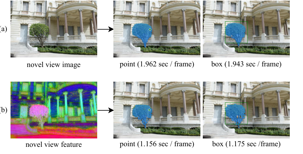
SAM from any view: render the SAM feature map at a novel pose and feed it to the SAM decoder directly (skipping the SAM image encoder) with a point or box prompt.
Language-guided editing: query the field with a CLIP text embedding to score each Gaussian, then build a Gaussian mask by soft (threshold), hard (argmax), or hybrid selection, and edit by updating opacity and color: extraction (keep the selected opacity, zero the rest), deletion (zero the selected opacity), or recoloring. Editing operates on the 3D Gaussians, so it stays 3D-consistent and can handle occluded parts.

6. Experiments

Datasets: Replica (indoor, semantic labels), LLFF, and editing scenes from NeRF-DFF / LERF / Deep Blending. Teachers: CLIP-LSeg (segmentation and editing) and SAM (promptable segmentation).

6.1 Novel-View Semantic Segmentation

Image quality (Table 1): adding the feature (and the speed-up module) slightly improves RGB over vanilla 3DGS; distilling features does not degrade the radiance field (5K training iterations, rendered feature dim 128).

Method	PSNR ↑ (±s.d.)	SSIM ↑ (±s.d.)	LPIPS ↓ (±s.d.)
Ours (w/ speed-up)	37.012 (±0.07)	0.971 (±5.3e-4)	0.023 (±2.9e-4)
Ours	36.915 (±0.05)	0.970 (±5.7e-4)	0.024 (±1.1e-3)
Base 3DGS	36.133 (±0.06)	0.965 (±1.5e-4)	0.033 (±1.2e-3)

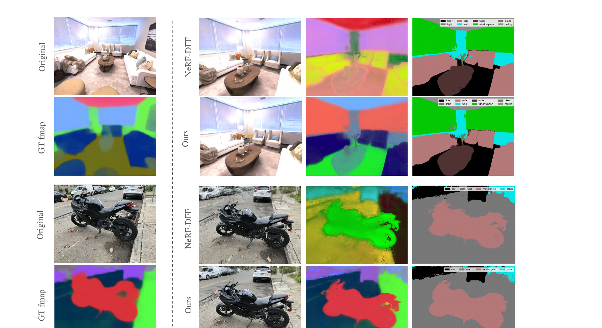
Segmentation (vs NeRF-DFF, Table 2): higher mIoU and accuracy than the NeRF-based feature field; the speed-up module more than doubles feature-render FPS (6.84 -> 14.55) at near-equal mIoU. Inference is about 1.66x faster than NeRF-DFF at feature dim 128.

Method	mIoU ↑	accuracy ↑	FPS ↑
Ours (w/ speed-up)	0.782	0.943	14.55
Ours	0.787	0.943	6.84
NeRF-DFF	0.636	0.864	5.38

Novel-view semantic segmentation (LSeg) on Replica (top) and LLFF (bottom) (paper Fig. 3). Columns: original image / GT feature map, then NeRF-DFF and Ours, each showing rendered RGB, PCA-colored feature, and segmentation. Feature 3DGS renders sharper features and cleaner masks.

6.2 Segment Anything from Any View

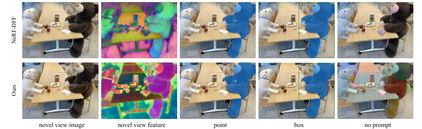
Decoding the rendered SAM feature directly (rather than re-encoding the rendered RGB) is up to about 1.7x faster end to end at equivalent mask quality, and gives finer instance boundaries than NeRF-DFF.

SAM segmentation, naive vs feature-field decoding (paper Fig. 4). (a) run the full SAM encoder + decoder on the rendered novel-view image; (b) decode the rendered SAM feature directly (SAM decoder only). Near-equivalent mask quality, up to about 1.7x faster end to end (per-frame times shown).

Novel-view SAM segmentation vs NeRF-DFF (paper Fig. 5). Top row NeRF-DFF, bottom row Feature 3DGS; columns: novel-view image, rendered feature (PCA-colored), and point / box / no-prompt masks. Feature 3DGS renders sharper features and finer-grained masks (e.g. the bear's leg boundary).

6.3 Language-Guided Editing

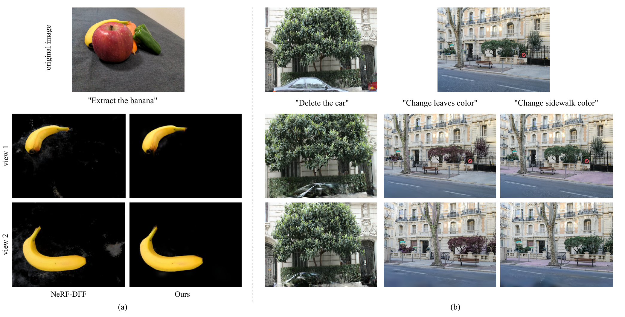
Extract an object even when occluded (3D awareness), delete an object while preserving the background via opacity updates, and recolor a target category without touching adjacent objects.

Language-guided editing by querying the 3D feature field (paper Fig. 6). (a) extract the banana, occluded by an apple in the original image, across two views, vs NeRF-DFF; (b) delete the car with background preserved, and recolor leaves / sidewalk without touching the stop sign.

6.4 Ablations

Rendered feature dimension (LSeg teacher): training time and quality both rise with the rendered dim ( $N$ = 8 / 16 / 32 / 64 / 128 / 256 / 512 gives mIoU 0.354 / 0.493 / 0.709 / 0.774 / 0.783 / 0.791 / 0.790). mIoU saturates by 128, and dim 128 trains about 2.4x faster than dim 256 for near-equal quality, so 128 is the default. SAM feature-render FPS likewise falls from 64.7 (dim 8) to 8.3 (dim 256) as the dimension grows.

Speed-up module: including it roughly halves render time with negligible quality loss, and can be dropped without hurting downstream tasks.

7. Discussion and Conclusion

Integrating 3DGS with 2D feature-field distillation gives an explicit, editable, promptable 3D scene representation: it renders full-resolution features fast, distills with equal loss weighting (no NeRF-DFF $\gamma$ -sensitivity), leaves RGB quality intact (slightly improved), and unlocks semantic segmentation, SAM promptable segmentation from any view, and 3D-consistent language editing from one representation.

Limitations (paper-stated)

Performance is capped by the teacher: the student only sees the teacher's features, and teacher imperfections propagate.
Inherited from 3DGS, noise-inducing floaters can degrade results.
On complex scenes with many small or similar adjacent objects, prompt-based selection can be imperfect (coarse SAM masks; incomplete deletions), which the paper attributes mainly to low teacher-feature quality rather than the Gaussian representation. The paper states no explicit future-work agenda beyond addressing these.

Personal comment: the "supercharging" gains are largely inherited from 3DGS's own speed, so the fair comparison is against NeRF-based distillation (NeRF-DFF), where the +23% mIoU and about 2.7x speed are convincing. The baseline is NeRF-DFF, not the 2D teacher it distills: since the student's only supervision is the teacher, the teacher is its ceiling (multi-view fusion can make the rendered field more view-consistent than a single-frame 2D prediction, but does not exceed the teacher's semantic quality). The speed-up module's low-dim-then-lift trick is the most practically reusable contribution. This is my own reading, not a claim in the paper.

Table of Contents