Description: Magic Moments paper note — reinterprets volume rendering as a stochastic process to derive closed-form higher-order moments (variance) without extra training; applies to both NeRF and 3DGS (2 ms/frame real-time UQ on 3DGS), covering color/depth/semantics
My Notion Note ID: K2E-B-G6-6
Created: 2026-07-01
Updated: 2026-07-13
License: Free to share: please credit Yu Zhang and link back to yuzhang.io

1. Summary

Title: These Magic Moments: Differentiable Uncertainty Quantification of Radiance Field Models Authors: P. Ewen, H. Chen, S. Isaacson, J. Wilson, K. A. Skinner, R. Vasudevan Paper: arXiv:2503.14665 (2025) Github: no public code release found (as of 2026-07)

University of Michigan, 2025. Proposes differentiable uncertainty quantification (UQ) for radiance fields (NeRF and 3DGS) — no model modification or additional training required.

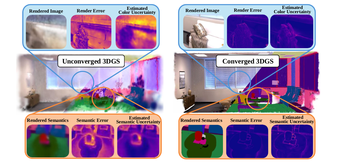
Core insight: Volume rendering is inherently stochastic — the position where a photon collides with a particle along a ray is a random variable. The rendered pixel value $\rho$ is therefore a random variable whose expectation equals the standard rendering equation. Following the same logic, integrating $\rho^j$ (the $j$ -th power) yields the $j$ -th moment $\mathbb{E}[\rho^j]$ ; variance then follows as $\text{Var}[\rho] = \mathbb{E}[\rho^2] - \mathbb{E}[\rho]^2$ — no extra training or parameters needed.

Key results:

Color variance correlates more strongly with rendering error than all baselines (FisherRF, CF-NeRF, 3DGS Ensemble) on every dataset (Table 1); depth variance leads all baselines on TUM and beats Bayes' Rays on Spearman/Kendall (Blender), though its Blender Pearson (0.718) is slightly below Bayes' Rays (0.758). Semantic variance has no baseline (Table 3 is "Ours" only)
2 ms/frame (3DGS); FisherRF requires 13679 ms on the same scene (6800× faster)
Color variance as NBV criterion outperforms FisherRF on Blender and TUM datasets

Uncertainty maps for an unconverged vs. converged 3DGS scene: rendered image, render error, and estimated color/semantic uncertainty. Estimated uncertainty closely tracks true render error in both regimes.

2. Key Contributions

Closed-form higher-order moments: Proves that the $j$ -th moment $\mathbb{E}[\rho^j]$ can be computed with the same integral form as standard rendering — replace integrand $\rho$ with $\rho^j$ ; Monte Carlo approximation for NeRF, direct extension of alpha blending for 3DGS
Unified framework: Same formula applies unchanged to color, depth, and semantic outputs, and to both NeRF and 3DGS model families
Zero training overhead: Post-hoc method — any trained model is used directly for UQ with no fine-tuning
Downstream validation: Color variance for NBV selection outperforms FisherRF; variance-guided active ray sampling (mean ray variance per cell of a 2D image grid) matches iMAP (which requires ground-truth error) performance

3. Method

3.1 Probabilistic Volume Rendering Framework

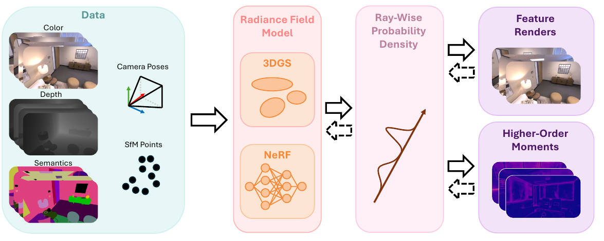
Classical local illumination model: scene = dense cloud of opaque emissive particles; a photon traveling along a ray collides at some position $s$ and renders that particle's color. Collision position is a random variable with probability density proportional to $\sigma(\mathbf{r}(s))$ (volume density).

Transmittance $T_a^b[\mathbf{r}]$ — probability of traveling from $a$ to $b$ along ray $\mathbf{r}$ without collision:

T_a^b[\mathbf{r}] = \exp\!\Bigl(-\int_a^b \sigma(\mathbf{r}(s))\,\mathrm{d}s\Bigr)

$T_{z_n}^s[\mathbf{r}]\,\sigma(\mathbf{r}(s))$ is the probability density of collision at position $s$ (surviving from near clip $z_n$ to $s$ , then hitting at $s$ ).

Standard rendering equation (= expectation of $\rho$ ):

\mathbb{E}[\rho] = \int_{z_n}^{z_f} \rho(\mathbf{r}(s))\,\sigma(\mathbf{r}(s))\,T_{z_n}^s[\mathbf{r}]\,\mathrm{d}s

$\rho$ = color, depth, or semantic embedding; $z_n, z_f$ = near/far clip planes.

3.2 Higher-Order Moment Derivation

Replace $\rho(s)$ with $\rho(s)^j$ in the expectation integral → $j$ -th moment:

\mathbb{E}[\rho^j] = \int_{z_n}^{z_f} \rho(\mathbf{r}(s))^j\,\sigma(\mathbf{r}(s))\,T_{z_n}^s[\mathbf{r}]\,\mathrm{d}s

Variance:

\text{Var}[\rho] = \mathbb{E}[\rho^2] - \mathbb{E}[\rho]^2

Derivation makes no distributional assumption on $\rho$ . Higher central moments (skewness, kurtosis, etc.) follow analogously, or parametric distributions can be fit via moment matching.

3.3 NeRF Implementation

Discretize the continuous integral as a Monte Carlo sum over $N$ uniform intervals. Let $T_i = \exp(-\sum_{k<i}\sigma_k\delta_k)$ , $\delta_i = t_{i+1}-t_i$ (inter-sample spacing).

Expected value (= standard NeRF rendering):

\mathbb{E}[\rho] = \sum_{i=0}^{N} T_i\,c_i\,(1-\exp(-\sigma_i\delta_i))

$j$ -th moment (replace $c_i$ with $c_i^j$ , same weights):

\mathbb{E}[\rho^j] = \sum_{i=0}^{N} T_i\,c_i^j\,(1-\exp(-\sigma_i\delta_i))

No additional forward pass — just one extra weighted sum over the same network outputs $c_i, \sigma_i$ .

3.4 3DGS Implementation

3DGS projects 3D Gaussians onto the image plane via alpha blending — equivalent to marginalizing a per-ray Gaussian mixture model (GMM). The effective alpha of the $i$ -th Gaussian at pixel $x$ , direction $d$ :

\tilde{\alpha}_i(x, d) = \alpha_i \cdot \exp\!\Bigl(-\tfrac{1}{2}\|x-\boldsymbol{\mu}_i(d)\|^2_{\boldsymbol{\Sigma}_i^{-1}(d)}\Bigr)

$\boldsymbol{\mu}_i(d), \boldsymbol{\Sigma}_i(d)$ = 2D projected mean and covariance of the $i$ -th Gaussian; $\alpha_i$ = opacity.

Expected value (= standard 3DGS rendering):

\mathbb{E}[\rho] = \sum_{i\in I}\rho_i\,\tilde{\alpha}_i(x,d)\prod_{k<i}(1-\tilde{\alpha}_k(x,d))

$I$ = depth-sorted Gaussian set.

$j$ -th moment (replace $\rho_i$ with $\rho_i^j$ , identical weights):

\mathbb{E}[\rho^j] = \sum_{i\in I}\rho_i^j\,\tilde{\alpha}_i(x,d)\prod_{k<i}(1-\tilde{\alpha}_k(x,d))

Near-zero overhead — computed in the same forward pass as standard rendering; only requires storing the extra weighted sum of $\rho_i^2$ in the rasterizer.

$\rho$ can be: RGB color ( $j=2$ → color variance), depth ( $j=2$ → depth variance), or semantic embedding vector ( $j=2$ → per-channel semantic variance).

4. Experiments & Results

Baselines:

FisherRF — Fisher information-based UQ for 3DGS
Bayes' Rays — spatial perturbation UQ for NeRF
CF-NeRF — conditional flow-based NeRF uncertainty
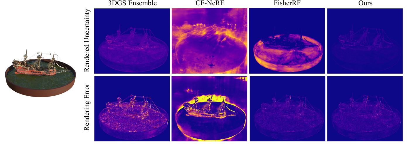
3DGS Ensemble — variance of 10 independently trained 3DGS models

Datasets: Blender (synthetic objects), Mip360 (real unbounded indoor + outdoor scenes), TUM (indoor RGB-D)

Color variance vs. rendering error correlation (Table 1):

Method	Blender $\tau_p$	Blender Time	Mip360 $\tau_p$	Mip360 Time	TUM $\tau_p$	TUM Time
FisherRF	0.580	13679 ms	0.527	156071 ms	0.482	46769 ms
CF-NeRF	0.307	180718 ms	0.113	5329000 ms	—	—
3DGS Ensemble	0.663	29 ms	0.398	79 ms	0.434	237 ms
Ours	0.716	2 ms	0.885	7 ms	0.781	20 ms

$\tau_p$ = Pearson correlation coefficient (higher = better). On Mip360, ours reaches 0.885 while FisherRF scores only 0.527 (and $\tau_s = -0.007$ , effectively useless). 3DGS Ensemble is competitive in correlation but an order of magnitude slower (11–15× across datasets).

Depth variance correlation (Table 2, Blender + TUM):

Method	Blender $\tau_p$	Time	TUM $\tau_p$	Time
FisherRF	0.572	13679 ms	0.546	46769 ms
Bayes' Rays	0.758	45221 ms	0.596	46399 ms
CF-NeRF	−0.086	180718 ms	—	—
3DGS Ensemble	0.362	29 ms	0.204	237 ms
Ours	0.718	2 ms	0.671	20 ms

On TUM, ours leads all baselines across all metrics. On Blender, Pearson $\tau_p$ (0.718) is slightly below Bayes' Rays (0.758), but Spearman/Kendall (0.792/0.700) substantially exceed Bayes' Rays (0.473/0.364) — at orders-of-magnitude lower latency. 3DGS Ensemble depth Pearson is poor on both datasets (0.362 / 0.204); CF-NeRF's depth variance is anti-correlated on Blender (−0.086) and did not converge on TUM.

Next-best-view selection (Table 4, 12-view Blender + 300-view TUM):

Method	Blender PSNR ↑	LPIPS ↓	Time ↓	TUM PSNR ↑	LPIPS ↓	Time ↓
Random	23.072	0.162	—	19.175	0.382	—
ActiveNeRF	14.115	0.280	1014 s	10.834	0.613	1272.8 s
FisherRF	23.658	0.148	13.8 s	18.978	0.388	47.4 s
Ours (depth var.)	22.867	0.185	0.6 s	18.946	0.388	0.9 s
Ours (color var.)	23.944	0.128	0.6 s	19.191	0.382	0.9 s

Compared against two SOTA baselines (ActiveNeRF and FisherRF), color variance NBV outperforms FisherRF on Blender (PSNR +0.3 dB, LPIPS −0.020) at 23× lower planning time; ActiveNeRF collapses on both datasets (Blender PSNR 14.1, TUM 10.8) at ~1000× the planning time. Depth variance NBV is substantially weaker (Blender PSNR 22.9 vs. 23.9, even below the Random baseline at 23.1) — expected, since PSNR/SSIM/LPIPS measure color quality and color variance aligns better with the optimization objective.

Active ray sampling: image is divided into a 2D grid; the mean ray variance is computed per cell (iMAP instead uses mean rendering error per cell), and high-variance cells get more sampled rays. This variance-guided sampling matches iMAP (ground-truth error-guided) across all Blender scenes, both substantially outperforming the uniform-sampling NeRF baseline.

5. Ablation & Discussion

Why color variance beats depth variance for NBV? NBV evaluation metrics (PSNR/SSIM/LPIPS) directly measure color rendering quality → color variance is better aligned with the optimization objective.

Why does FisherRF fail on Mip360 ( $\tau_s=-0.007$ )? FisherRF assumes a linearized rendering model with a Gauss-Newton approximation. In unbounded/large-scale scenes where the number of Gaussian basis functions is unconstrained, it severely overestimates uncertainty. Mip360 is a typical unbounded scene.

Limitation with unconverged models: As shown in Fig. 1, variance maps from a partially trained 3DGS are blurry because the model itself is not yet accurate. Variance reflects the model's intrinsic aleatoric uncertainty about its own output — it is not an external noise estimator.

Pixel independence approximation: NBV experiments sum per-pixel variances, ignoring correlations that arise because a single Gaussian influences multiple pixels. A rigorous joint uncertainty estimate would require computing the uncertainty of the joint distribution; the current approximation already outperforms baselines in practice but is theoretically incomplete.

6. Strengths / Limitations / Future Work

Strengths

Elegant derivation: $j$ -th moment formula is structurally identical to the rendering equation — just replace $\rho$ with $\rho^j$
Zero extra training: plug into any pretrained NeRF or 3DGS, no ensemble, no architecture changes
Unified across modalities: color/depth/semantics share one formula; FisherRF is limited to color+depth
Real-time speed: 2 ms vs. FisherRF 13679 ms (3DGS, Blender) — viable for online robot planning

Limitations

Requires model convergence: variance reflects the model's current fit quality; unreliable for undertrained models
Low semantic correlation (Mip360 $\tau_p=0.18$ ): CLIP-LSeg view-inconsistency noise drowns the semantic variance signal; closed-set semantics (SGS-SLAM) suffer boundary artifacts
Pixel independence approximation: ignores inter-Gaussian covariance; rigorous joint uncertainty is future work
Limited edge over Random baseline (TUM): the paper notes the Random baseline performs surprisingly well on TUM. Its homogeneity/entropy argument targets FisherRF specifically — TUM's homogeneous surfaces (walls, desks) yield low entropy, so FisherRF instead over-selects close-up views of small high-entropy objects, hurting it; the strong Random result leaves all methods with only a narrow margin

Future Work

True joint pixel uncertainty (beyond the independence approximation) — the only future direction the paper's conclusion names
(Note-author idea, not in paper) Combine with visibility fields (e.g. GAVIS) to improve UQ in unexplored regions

References

Ewen, P., Chen, H., Isaacson, S., Wilson, J., Skinner, K. A., & Vasudevan, R. (2025). These Magic Moments: Differentiable Uncertainty Quantification of Radiance Field Models. arXiv:2503.14665.
Jiang, W., Lei, B., & Daniilidis, K. (2023). FisherRF: Active view selection and uncertainty quantification for radiance fields using Fisher information. arXiv:2311.17874.
Goli, L., et al. (2024). Bayes' Rays: Uncertainty quantification for neural radiance fields. CVPR 2024.
Shen, J., Agudo, A., Moreno-Noguer, F., & Ruiz, A. (2022). Conditional-Flow NeRF: Accurate 3D modelling with reliable uncertainty quantification. ECCV 2022. (The Magic Moments paper's tables mis-cite this baseline as ref [49] Yan et al. "CF-NeRF: Camera parameter free…", AAAI 2024 — an unrelated method — but its related-work and experiment text describe the conditional continuous-flow uncertainty method, i.e. this Shen et al. paper.)
Sünderhauf, N., Abou-Chakra, J., & Miller, D. (2023). Density-aware NeRF Ensembles: Quantifying predictive uncertainty in neural radiance fields. ICRA 2023.
3D Gaussian Splatting note: 3DGS representation fundamentals
GAVIS note: visibility field-driven active mapping

Table of Contents