Description: Transformer paper note — the sequence model that drops recurrence and convolution entirely and computes representations purely from (self-)attention: scaled dot-product + multi-head attention, positional encodings, encoder-decoder stacks; new WMT'14 SOTA BLEU at a fraction of the training cost, and the backbone every later architecture (BERT, ViT, CroCo, DUSt3R, VGGT) builds on
My Notion Note ID: K2F-B-1
Created: 2026-08-02
Updated: 2026-08-02
License: Free to share: please credit Yu Zhang and link back to yuzhang.io

1. Summary

Title: Attention Is All You Need Authors: A. Vaswani, N. Shazeer, N. Parmar, J. Uszkoreit, L. Jones, A. N. Gomez, Ł. Kaiser, I. Polosukhin (Google Brain / Google Research / U. Toronto) Paper: arXiv:1706.03762 (NIPS 2017 — pre-NeurIPS rename) Github: tensorflow/tensor2tensor (official reference implementation)

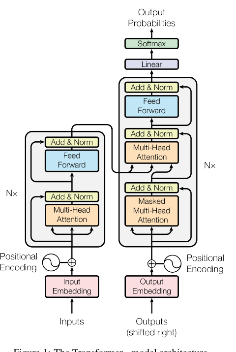
Transformer — a sequence transduction model built entirely on attention, with no recurrence (RNN) and no convolution. Originally for machine translation; it became the universal backbone of modern deep learning.

Core problem: RNN-based sequence models (LSTM/GRU seq2seq) are inherently sequential — computation at step $t$ needs the hidden state from $t-1$ , so training cannot be parallelized across positions and long sentences are slow. Attention was already used alongside RNNs to connect distant positions; the paper's bet is that attention alone suffices.

Key idea: replace recurrence with self-attention — every position attends to every other position in one step. This gives (a) full parallelism across positions and (b) a constant path length between any two tokens, so long-range dependencies are easy to learn (an RNN needs $O(n)$ steps to connect tokens $n$ apart; self-attention needs $O(1)$ ).

The building blocks:

Scaled dot-product attention — the core operation: weight each value by the (scaled, softmaxed) dot product of a query with each key.
Multi-head attention — run several attention functions in parallel in different learned subspaces, so the model attends to different kinds of relations at once.
Positional encoding — since attention is permutation-invariant, inject token order via fixed sinusoids added to the embeddings.
Everything wrapped in residual connections + layer normalization, with a position-wise feed-forward network per layer.

Main results: new state of the art on WMT'14 — 28.4 BLEU EN→DE (big model, +2.0 over the best prior including ensembles) and 41.8 BLEU EN→FR — trained in 3.5 days on 8 GPUs, a small fraction of prior SOTA training cost.

Transformer architecture: a stack of N encoder layers (multi-head self-attention + feed-forward, each wrapped in residual + layer-norm) on the left; a stack of N decoder layers on the right adding masked self-attention and encoder-decoder cross-attention, ending in a linear + softmax over the vocabulary.

2. Key Contributions

The Transformer architecture — the first transduction model relying entirely on self-attention, no RNN/CNN.
Scaled dot-product + multi-head attention — a cheap, highly parallel attention formulation with the $1/\sqrt{d_k}$ scaling that keeps softmax gradients healthy at large dimension.
Sinusoidal positional encoding — order information without recurrence, chosen so relative offsets are linear functions of position (may extrapolate to longer sequences).
Demonstrated that parallelism + short paths win — SOTA translation at a fraction of training cost, launching the "attention-only" era.

3. Method

3.1 Encoder–Decoder Stacks

Standard encoder–decoder: the encoder maps input tokens $(x_1,\dots,x_n)$ to continuous representations $z$ ; the decoder generates output $(y_1,\dots,y_m)$ one token at a time, auto-regressively (each new token conditions on previously generated ones).

Encoder: $N=6$ identical layers, each = [multi-head self-attention] + [position-wise feed-forward]. Each sub-layer is wrapped as $\text{LayerNorm}(x + \text{Sublayer}(x))$ (residual + layer-norm). All sub-layers and embeddings output dimension $d_\text{model}=512$ .
Decoder: $N=6$ layers, each adding a third sub-layer — multi-head attention over the encoder output (cross-attention). Its self-attention is masked so position $i$ can only attend to positions $< i$ , preserving the auto-regressive property (no peeking at future tokens).

3.2 Scaled Dot-Product Attention

Attention maps a query and a set of key–value pairs to an output = a weighted sum of the values, where each weight is a compatibility score between the query and that value's key. Packed into matrices $Q, K, V$ :

\text{Attention}(Q, K, V) = \text{softmax}\!\left(\frac{QK^\top}{\sqrt{d_k}}\right) V

$Q$ = queries, $K$ = keys (both dimension $d_k$ ), $V$ = values (dimension $d_v$ ); $QK^\top$ = all query–key dot products, softmax over each row gives the attention weights, which mix the values.

Why the $1/\sqrt{d_k}$ scaling: for large $d_k$ the dot products grow in magnitude (with unit-variance components, $q\cdot k$ has variance $d_k$ ), pushing softmax into saturated regions with tiny gradients. Dividing by $\sqrt{d_k}$ counteracts this. Dot-product attention (vs additive attention) is chosen because it's a single matrix multiply — fast and memory-efficient.

3.3 Multi-Head Attention

Instead of one attention over $d_\text{model}$ -dim vectors, linearly project $Q,K,V$ into $h$ lower-dim subspaces, attend in each in parallel, concatenate, and project back:

\text{MultiHead}(Q,K,V) = \text{Concat}(\text{head}_1,\dots,\text{head}_h)\,W^O, \qquad \text{head}_i = \text{Attention}(QW_i^Q, KW_i^K, VW_i^V)

$W_i^Q, W_i^K \in \mathbb{R}^{d_\text{model}\times d_k}$ , $W_i^V \in \mathbb{R}^{d_\text{model}\times d_v}$ , $W^O \in \mathbb{R}^{h d_v \times d_\text{model}}$ are learned projections. Different heads attend to different representation subspaces at once — a single head would average these together and lose that. The paper uses $h=8$ heads with $d_k = d_v = d_\text{model}/h = 64$ , so total cost ≈ single full-dim head.

3.4 Where Attention Is Used

Three uses of multi-head attention:

Encoder self-attention — Q, K, V all from the previous encoder layer; every position attends to all positions.
Decoder masked self-attention — attends to earlier decoder positions only; illegal (future) connections masked to $-\infty$ before softmax.
Encoder–decoder (cross-)attention — queries from the decoder, keys/values from the encoder output; lets each decoder position attend over the whole input. (This cross-attention is the direct ancestor of the "global attention across views" in multi-view 3D transformers.)

3.5 Feed-Forward, Embeddings, Positional Encoding

Position-wise FFN — applied identically to each position: two linear layers with ReLU, $\text{FFN}(x) = \max(0, xW_1 + b_1)W_2 + b_2$ ; inner dimension $d_{ff} = 2048$ .
Embeddings — learned token embeddings of dim $d_\text{model}$ ; input embeddings, output embeddings, and the pre-softmax projection share weights (embeddings scaled by $\sqrt{d_\text{model}}$ ).
Positional encoding — added to embeddings so the model knows token order. Fixed sinusoids of geometric wavelengths ( $2\pi$ to $10000\cdot2\pi$ ):

PE_{(pos, 2i)} = \sin\!\left(\frac{pos}{10000^{2i/d_\text{model}}}\right), \qquad PE_{(pos, 2i+1)} = \cos\!\left(\frac{pos}{10000^{2i/d_\text{model}}}\right)

$pos$ = position, $i$ = dimension index. Chosen so $PE_{pos+k}$ is a linear function of $PE_{pos}$ for any fixed offset $k$ (easy relative-position attention) and to potentially extrapolate beyond training lengths. Learned positional embeddings gave near-identical results (Table 3 row E).

4. Why Self-Attention

Three desiderata compared across layer types (Table 1; $n$ = sequence length, $d$ = representation dim):

Layer type	Complexity / layer	Sequential ops	Max path length
Self-Attention	$O(n^2 \cdot d)$	$O(1)$	$O(1)$
Recurrent	$O(n \cdot d^2)$	$O(n)$	$O(n)$
Convolutional	$O(k \cdot n \cdot d^2)$	$O(1)$	$O(\log_k n)$
Self-Attention (restricted, neighborhood $r$ )	$O(r \cdot n \cdot d)$	$O(1)$	$O(n/r)$

Self-attention wins on sequential operations (fully parallel, $O(1)$ ) and path length ( $O(1)$ — any two positions directly connected). It is also cheaper than recurrence per layer when $n < d$ (usually true for sentence representations). Bonus: attention heads are somewhat interpretable, appearing to learn syntactic/semantic structure.

5. Experiments & Results

Task / data: WMT'14 EN→DE (4.5M sentence pairs, ~37k shared BPE vocab) and EN→FR (36M sentences, 32k word-piece vocab). Trained on 8 × NVIDIA P100 GPUs. Base: 100k steps (~12 h); Big: 300k steps (~3.5 days). Adam with $\beta_1=0.9, \beta_2=0.98, \epsilon=10^{-9}$ ; learning rate warmup over 4000 steps then inverse-sqrt decay; residual dropout 0.1; label smoothing 0.1. Beam size 4, length penalty 0.6.

Translation BLEU (newstest2014):

Model	EN→DE BLEU	EN→FR BLEU	Train FLOPs (EN-DE)
GNMT + RL (ensemble)	26.30	41.16	~1.8·10²⁰
ConvS2S (ensemble)	26.36	41.29	~7.7·10¹⁹
Transformer (base)	27.3	38.1	3.3·10¹⁸
Transformer (big)	28.4	41.8	2.3·10¹⁹

(FLOPs shown for EN-DE; the baselines' EN-FR training cost is ~6× higher (~10²¹). Transformer rows report a single combined FLOPs value.)

The big model sets a new EN→DE SOTA at 28.4 (+2.0 BLEU over the best prior, ensembles included) and EN→FR 41.8 (Table 2; note §6.1's prose quotes 41.0 — an in-paper inconsistency), both at far lower training cost. Even the base model beats all prior published single models.

Ablations (Table 3, newstest2013): single-head attention is 0.9 BLEU worse than $h=8$ , but too many heads also hurt; shrinking $d_k$ hurts (dot-product compatibility isn't trivial); bigger models and dropout both help; learned vs sinusoidal positional encodings ≈ identical. Config: base = 65M params; big = $d_\text{model}$ 1024, $d_{ff}$ 4096, $h$ 16, 213M params.

6. Strengths / Limitations / Legacy

Strengths

Removed the sequential bottleneck of RNNs → massively parallel training and short gradient paths; this is the reason large-scale pretraining became feasible.
Conceptually minimal: attention + FFN + residual/LN + positional encoding, and it generalizes far beyond translation.
Strong empirical case (SOTA at lower cost) plus clean ablations isolating each design choice.

Limitations

$O(n^2)$ attention in sequence length — quadratic memory/compute makes very long sequences expensive (spawning a whole line of "efficient Transformer" work).
Fixed context; no built-in notion of locality or 2D structure — inductive bias must be learned from data (which is exactly why ViT later needs huge datasets).
Positional encoding is a bolt-on rather than intrinsic.

Legacy (why this note is the root of the reading arc)

BERT / GPT — encoder-only / decoder-only Transformers for language.
ViT — applies the encoder verbatim to image patches; the entire vision-transformer lineage follows.
CroCo → DUSt3R → VGGT — cross-view and multi-view 3D built on Transformer encoders + cross-attention; the "global attention across views" that VGGT relies on is this paper's cross-attention generalized to many images.

References

Vaswani, A., Shazeer, N., Parmar, N., Uszkoreit, J., Jones, L., Gomez, A. N., Kaiser, Ł., & Polosukhin, I. (2017). Attention Is All You Need. NeurIPS. arXiv:1706.03762, code. — source paper (Fig. 1 architecture above)
Bahdanau, D., Cho, K., & Bengio, Y. (2015). Neural Machine Translation by Jointly Learning to Align and Translate. ICLR. — additive attention alongside RNNs; the attention this paper makes standalone
Hochreiter, S., & Schmidhuber, J. (1997). Long Short-Term Memory. Neural Computation. — the recurrent baseline Transformers replace
Ba, J. L., Kiros, J. R., & Hinton, G. E. (2016). Layer Normalization. — the normalization used around each sub-layer
ViT: the direct application of this encoder to vision, next in the reading arc

Transformer: Attention Is All You Need

Table of Contents